Courses: Introduction to GoldSim:
Unit 8 - Representing Complex Dynamics: Loops and Delays
Lesson 10 - Modeling Material Delays
Material Delay elements are intended to be used to simulate delays in the physical movement (flow) or in some cases the change of state (e.g., eggs to chickens) of material within a system. These delays often have a critical impact on the dynamic behavior of systems.
You would use a Material Delay element to simulate processes like the movement of parts on a conveyor belt, the flow of water through a pipeline, the movement of cars from one location to another, and the movement of letters through the mail system.
Material is conserved as it moves through a Material Delay. In some cases, the material may be dispersed while in transit. For example, if you send 100 letters all at once, they will not be delivered at the same time. Rather, there will be some variability in the time at which they are delivered. In other cases, the material is not dispersed. If a conveyor belt moves at a fixed speed, there will be no variability in the transit times for material that is loaded onto the conveyor. Similarly, if water flows through a pipeline, for the most part it moves as a “plug flow” and there is no variability in the transit time for water entering the pipeline.
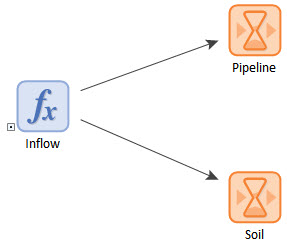
In order to understand how a Material Delay works, let’s open a simple pre-built model (you will do several Exercises using Material Delays in the next two Lessons). To do so, go to the “Examples” subfolder of the “Basic GoldSim Course” folder you should have downloaded and unzipped to your Desktop, and open a model file named Example8_MaterialDelay.gsm. The model will look like this:
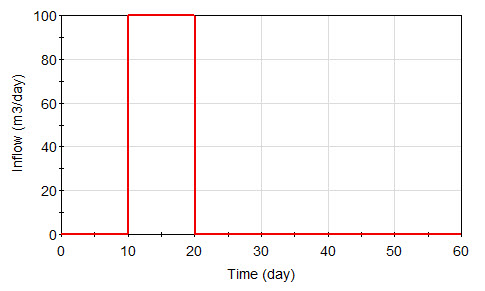
The Inflow element represents a flow rate that is equal to 100 m3/day between 10 days and 20 days, and is zero otherwise:
The other two elements are Material Delay elements. Open the one named Pipeline:
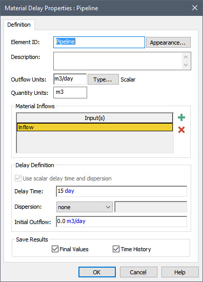
The element conceptually represents a pipeline through which the water is flowing. You will note that similar to the Pool element, the Material Delay element requires two sets of units (Outflow Units and Quantity Units). The Outflow Units must have the same dimensions as the Material Inflows to the Delay. So if the inflow is a mass rate (mass/time), the Outflow Units must be a mass rate. In our example, the inflow (and hence the outflow) is a volumetric flow rate, so the Outflow Units are specified as m3/day. The Quantity Units must therefore be a volume. In this case they are specified as m3, but they could have been specified as another unit of volume, such as gallons or liters. As we shall see, these are used as the display units for the two outputs of the Material Delay: the outflow (the primary output), and the amount of material in transit (a secondary output).
Material Delay elements require one or more Material Inflows to be specified. Material Inflows are specified by pressing the Add button (the plus sign), and selecting an output from the browser that is displayed. In this case, there is a single Material Inflow - the element named “Inflow”.
The Delay Time determines how long it takes to transit the Delay. In this case, it takes 15 days.
Let’s close this element and open the element named Soil:
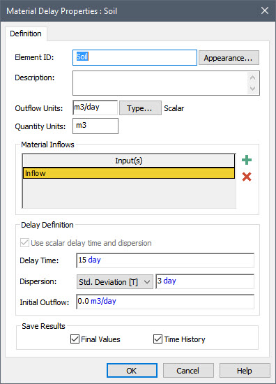
The element conceptually represents a column of soil through which the water is flowing. If you compare it to the Pipeline element, you will notice that they are identical with one exception: Soil has a defined Dispersion (specified as in terms of a Standard Deviation and equal to 3 days). The purpose of this is to represent the fact that unlike the Pipeline, when water moves through the soil column the flow is dispersed, “smoothed”, or “smeared” such that the outflow at any point is a weighted average of the inflow at previous times.
Note: The degree of Dispersion can be represented in two different ways: by specifying a “Standard Deviation”, or by specifying an “Erlang n”. The GoldSim Help system explains how one relates to the other.
Note: If you were really interested in modeling the flow of water though a soil column, you can imagine that the Delay Time and Dispersion would be defined as functions of the hydrogeological properties of the soil.
Run the model and double-click on the Result element to plot the Inflow and the two outflows (from the Pipeline and from the Soil):
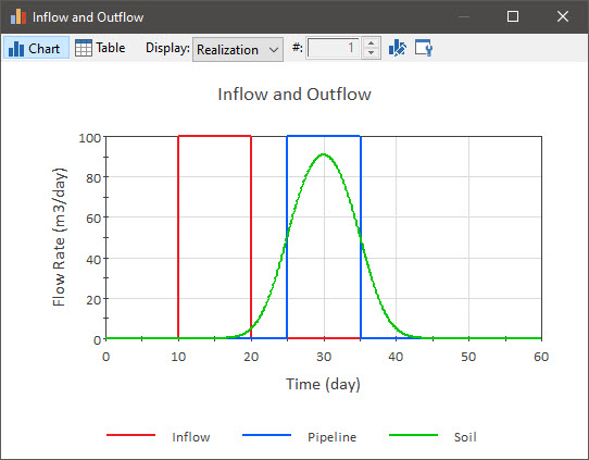
It should now be obvious exactly what a Material Delay does. The black curve shows the Inflow. The red curve shows the outflow from the Pipeline, which is delayed with no dispersion. The outflow begins exactly 15 days after the Inflow started, (and ends exactly 15 days after the Inflow stops).
The blue line shows the outflow from the Soil, which is delayed with dispersion. Instead of the outflow starting 15 days after the Inflow starts, the outflow begins much earlier: at about 7 days after the Inflow starts. Similarly, instead of the outflow ending 15 days after the Inflow stops, it ends about 22 days after the Inflow stops. That is, the outflow is dispersed.
Note that the area under each curve is the same since the material is conserved. (If you wanted to convince yourself of this, you could do so by routing the Inflow and the two outflows into three Reservoir elements that simply integrated the values.)
As pointed out above, Material Delay elements have two outputs: the outflow (the primary output) and the amount of material in transit (a secondary output). The chart above shows the primary output (the outflow). Let’s plot the secondary output (the Amount in Transit) for the Pipeline. To do so, left-click on the output port for the element, and then right-click on Amount_in_Transit and select Time History Result… It will look like this:
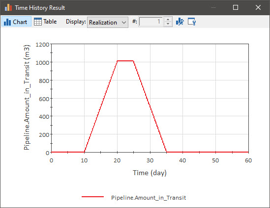
So what is happening here? At 10 days the Inflow begins and water is now present in the Pipeline. Between 10 days and 20 days, the water is moving through the Pipeline (and more water continues to flow in, increasing the amount of water in the Pipeline). At 20 days the Inflow stops. Between 20 days and 25 days the Inflow has stopped, but no water has yet been discharged (as the transit time is 15 days). Basically, a “slug” of water that entered between 10 days and 20 days is moving through the Pipeline. At 25 days, the Pipeline begins to discharge, and hence the amount of water in the Pipeline starts to decrease. By 35 days, all of the water (that entered between 10 days and 20 days) has been discharged, so that there is no water remaining in the Pipeline.
Note that the Amount_in_Transit started at zero. That is, the Pipeline was assumed to be empty at the beginning of the simulation. You can specify that the Delay begins the simulation with material already in transit by defining an Initial Outflow. By doing so, you are essentially assuming that the Delay begins the simulation “full”, with the initial amount in transit being defined as the Initial Outflow/Delay Time.