Lesson 11 - Representing Complex Diffusive Processes

In Lesson 4 we noted that the diffusive mass transfer rate between two Cells is equal to the product of the diffusive conductance and the concentration difference between the two Cells.  Assuming we have a single fluid on both sides of the diffusive mass flux link (and a porous medium Solid), the diffusive conductance is computed as follows:

τ n D_m A / Δx

where:

• D_m the diffusion coefficient (a property of the Fluid);
• τ is the tortuosity (a property of the Solid and its saturation);
• n is the porosity (a property of the Solid);
• A is the area through which the diffusion is taking place; and
• Δx  is the distance through which the diffusion is occurring.

Before concluding our discussion on the simulation of diffusion, in this Lesson we will briefly discuss several dimensionless factors that can be used to modify the diffusive conductance under certain circumstances.  Although you may never need to do this, exploring these factors and understanding their impact on diffusion rates provides insight into the process of diffusion and hence is worth examining here.

There are four dimensionless factors that can be used to modify the diffusive conductance:

• Relative Diffusivities;
• Available Porosities;
• Diffusivity Reduction Formula; and
• Relative Particulate Diffusivity

We have already briefly discussed the first dimensionless factor, but it is worth reiterating here. Recall that there are two inputs that define D_m: a Reference Diffusivity and Relative Diffusivities. The Reference Diffusivity is the diffusivity for a “standard” or “reference” species in the Fluid.  It has dimensions of area/time. Relative Diffusivities can then be specified for each species (or if you are simulating isotopes, each element).  These are dimensionless values that all default to one. For a given species, the actual diffusion coefficient is equal to the Reference Diffusivity times the Relative Diffusivity for that species. Hence, if you keep all of the Relative Diffusivities at their default value of 1, all of the species will have the same diffusion coefficient (equal to the Reference Diffusivity). However, by specifying different Relative Diffusivities, you can have a different diffusivity for each species you are simulating (i.e., you can allow D_m to vary by species).  As we shall see below, the impact of changing the diffusivity is straightforward: it linearly affects the rate of diffusion.

The second  factor that can be specified to adjust the diffusive conductance pertains only  when modeling diffusion through a porous medium.  As such, it is a property of the porous medium (i.e., the Solid).  If you open a Solid dialog, and press the Advanced Properties… button, the following dialog will be displayed:

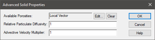
We are interested in the Available Porosities field. This represents the fraction of the pore volume within the Solid that is accessible to each species.  It effectively allows you, for the purpose of mass transport calculation, to make the porosity of the porous medium a function of the species.

Available Porosities can then be specified for each species (or if you are simulating isotopes, each element).  These are dimensionless values that all default to one. For a given species, the actual porosity that it sees is equal to the Porosity times the Available Porosity for that species. Hence, if you keep all of the Available Porosities at their default value of 1, all of the species will see the same porosity).

An available porosity less than 1 indicates that some of the pore volume is inaccessible for that species.  Implementing an available porosity which is less than 1 may be appropriate when simulating Cell Pathways involving media such as clay, where processes such as anion exclusion may be active. 

As we shall see below, the impact of specifying a fractional available porosity for a solid on mass transfer rates is complex:

• For diffusive mass flux links (and matrix diffusion zones) in which the Solid is specified as the porous medium, the effective diffusivity for the species of interest is multiplied (reduced) by the Available Porosity.
• The volume of water available to the species is reduced.  This in turn affects the concentration (and hence the concentration gradient for diffusive mass flux links).  Moreover, decreasing the volume of accessible water increases the retardation due to sorption (since all of the mass of the porous medium is still assumed to be available, but only a fraction of the water is).

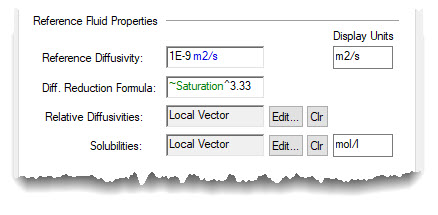
In our discussions thus far in this Unit, we have been concerned with diffusion through a single fluid (typically within a porous medium).  However, diffusion becomes much more complicated when the porous medium is only partially saturated (and hence you have two Fluids: water and air). To address this complication, Fluids have another property that impacts the diffusivity.  The Diffusivity Reduction Formula allows you to define how the effective diffusivity through the fluid is impacted by the fluid’s saturation level within any Cell pathways in which it is present.  This input is available just below the Reference Diffusivity on the Fluid dialog.

Physically, this term is intended to be less than or equal to 1 (it defaults to 1).  If the porous medium through which diffusion is occurring is saturated, this should be left at its default value of 1.  But if the porous medium is only partially saturated, you should enter a formula here. When used, this formula is intended to directly reference the fluid’s saturation level using a special variable called “Saturation”.  It must be referenced as “~Saturation” in the equation entered into the field, such as in the example below:

“Saturation” is what is known as a locally available property. Locally available properties derive their name from the fact that they may only be available, or they may take on different values (i.e., be over-ridden), in “locally available” parts of your model (e.g., in this case, within the Diffusivity Reduction Formula field).

The “Saturation” locally available property instructs GoldSim to internally compute the saturation of the fluid in the pathway (based on how you have defined the amounts of Fluids and Solids and their properties).

Conceptually, the Diffusivity Reduction Formula should equal 1 when the saturation is equal to 1 (and 0 when the saturation is equal to 0). As a result, one convenient form for the Diffusivity Reduction Formula is:

Diffusivity Reduction Formula = ~Saturation^X

As we shall see below, like the Available Porosities, the impact of saturation on the diffusion rate is complex. While the Diffusivity Reduction Formula (when defined appropriately as a function of saturation) reduces the effective diffusivity, a lower saturation changes the volume of water available.  This in turn affects the concentration (and hence the concentration gradient).  Moreover, decreasing the volume of water available increases the retardation due to sorption (since all of the mass of the porous medium is still assumed to be available, but only a fraction of the water is).

It is worthwhile at this point to briefly look at an Example model to view the effects of these three dimensionless variables (Relative Diffusivity, Available Porosity and Diffusivity Reduction Formula) on diffusion rates. To do so, go to the “Examples” subfolder of the “Contaminant Transport Course” folder you should have downloaded and unzipped to your Desktop, and open a model file named ExampleCT24_Adjusting_Diffusive_Conductance.gsm.

This model is very similar to the tube example we explored in Lesson 5 in which we simulated the diffusion of species through a tube that was filled with a porous medium and saturated (ExampleCT19_Diffusive_Tube.gsm).  However, several minor changes have been made for the purposes of comparing and contrasting the impacts of these dimensionless variables:

• To represent partial saturation, two different tubes were simulated (one saturated, one unsaturated).
• Four species were simulated (the first three were introduced into the saturated tube, and only the fourth was introduced into the unsaturated tube):
  • W (the base case)
  • X (Relative Diffusivity of 0.5)
  • Y (Available Porosity of 0.5)
  • Z (Saturation of 0.7, and Diffusivity Reduction Formula of ~Saturation^3.33 = 0.3)
• All four species were assigned a partition coefficient of 1E-4 m3/kg.

We won’t bother to explore the model here (although you are encouraged to do so) as the changes are straightforward.  Instead we will focus on the results. Run the model and open the “Release Rate” Time History Result element.  This shows the release rate out the end of the tube (recall that the boundary condition was zero concentration, similar to assuming diffusion into a rapidly flushed tank):

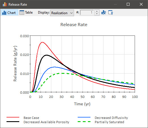
As can be seen, all three dimensionless variables slow the rate of diffusion, but in different ways:

• The most straightforward impact is that caused by the decreased relative diffusivity.  This linearly impacts the rate of diffusion.  In fact, the peak release rate for the species with the Relative Diffusivity of 0.5  (the blue curve) occurs exactly two times later than the base case.
• The impact of decreasing the available porosity is more complex.  Although the effective diffusivity for the species is reduced by the Available Porosity, the volume of water available to the species is also reduced. This in turn affects the concentration (and hence the concentration gradient for diffusive mass flux links).  In fact, in the absence of sorption, reducing the Available Porosity would have no impact on the release rate (the reduced diffusivity is exactly offset by the increased gradient). However, decreasing the volume of water available also increases the retardation due to sorption (since all of the mass of the porous medium is still assumed to be available, but only a fraction of the water is). And that is why in this Example, the species with decreased Available Porosity is delayed relative to the base case.
• The impact of decreasing the saturation is even more complex.  Although the effective diffusivity for the species is reduced by the Diffusivity Reduction Formula, the volume of water available to the species is also reduced. This in turn affects the concentration (and hence the concentration gradient for diffusive mass flux links).  In this case, however, the reduction in the effective diffusivity (by a factor of 0.3) is greater than the increase in the gradient due to the saturation change (since the Diffusivity Reduction Formula is smaller than the saturation due to the manner in which it was specified in this Example).  Hence, even in the absence of sorption, reducing the saturation here impacts the release rate.  Moreover, decreasing the saturation also increases the retardation due to sorption (since all of the mass of the porous medium is still assumed to be available, but only a fraction of the water is). And that is why in this Example, the species in the partially saturated tube has the greatest delay.

This example (and the others presented in this Unit) should make it very clear that diffusion, while conceptually simple, can be a very complex process indeed!

The final dimensionless variable we will briefly mention is the Relative Particulate Diffusivity. Like the Available Porosities, this a property of a Solid and can be found in the Advanced Properties dialog for a Solid:

In previous Units, we discussed that Solids could be suspended in Fluids. If species partition between the Fluids and the suspended Solid, they could then be transported on the suspended particulates. In Unit 7, Lesson 8 we discussed the advection of species via suspended Solids (moving with the Fluid). In addition to being advected, however, suspended particulates can also diffuse (and hence transport mass).

The Relative Particulate Diffusivity is a dimensionless number between 0 and 1 (it defaults to 1). Similar to the relative diffusivity for a species, the relative diffusivity for a particulate Solid is multiplied by the Reference Diffusivity of the corresponding Fluid to determine the actual diffusivity of the particulate form of the Solid in the Fluid.  Typically, this value would be much smaller than 1. It often would not apply at all for porous media, as most suspended particles would be filtered out (unless they were very small, such as colloids) and hence you would not specify any suspended solids at all in the system.