Lesson 2 - Understanding Dynamic Behavior

In a dynamic simulation, the system changes with time, and we are interested in looking forward in time to predict how the system will evolve (and understand what we might be able to do to change that behavior).

Systems can change with time due to external influences and/or internal influences. External influences on the evolution of a model are referred to as being exogenous.  Exogenous behavior is something that comes from “outside” the model and is not due to or explained by the model itself.  It is simply an external “forcing function”. For example, if you were modeling a company whose performance was strongly impacted by the price of a commodity (that the company had no control over), the commodity price would be an exogenous factor, in that it would be changing with time (and hence would make the company performance change with time).  The model of the company would not explain or impact the commodity price; the commodity price would just be an external input. Another example of an exogenous factor would be the rainfall rate in a model that was attempting to track the volume of water in a pond.  The model of the pond would not explain or impact the rainfall rate; the rainfall rate would just be an external input.

Internal influences on the evolution of a model are referred to as being endogenous. Endogenous behavior is something that comes from “inside” the model and is explained by the relationships within the model. That is, if a system evolves endogenously, it means that the model structure itself is causing the model variables to change with time.  The changes are not being driven from something “outside” the model.

Remembering these specific terms (exogenous and endogenous) is not important.  What is critical is that you understand the concept: systems can change with time due to external influences and/or internal influences. Some (very simple) systems may only exhibit exogenous behavior.  Many may be dominated by endogenous behavior.  Most real-world systems that you will model, however, are controlled by both endogenous and exogenous factors.  A little thought will convince you that this must indeed be the case. Because the “system” we are simulating will always be a very small subset of the universe, and this system is unlikely to be completely isolated from the rest of the universe, exogenous factors will always exist.  Moreover, any system worth taking the time to model would by definition have sufficient complexity to have at least some internal endogenous behavior.

Let’s look at several very simple systems to illustrate this.

First, let’s consider a system which we can model using this equation:

Result = X + Y

where X and Y are external to the system.  That is, the model simply adds two exogenous variables. If X and Y did not change with time, the model would exhibit no dynamic behavior at all (the Result would stay constant in time). However, if X and/or Y varied with time, then the model would indeed exhibit dynamic behavior.  It might, for example, look like this:

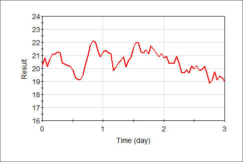
Although the result looks complex, it is important to understand that this is purely exogenous dynamic behavior. The model exhibits no endogenous behavior because in order to do so, the structure of the model (the functional relationships) would need to impart “memory” or “inertia” with regard to the past.  In this case, the Result is a function of the instantaneous values of X and Y (which are changing external to the model); as a result, the past values of X and Y have no impact whatsoever on the current value of Result. Hence, this simple model cannot generate endogenous behavior.

Now let’s consider a slightly more complex system (with a correspondingly more complex model that describes it). Recall the tank that we simulated back in Unit 4.  In that system, we were filling a tank with water via a hose, but the tank was leaking. Mathematically, we can model that system using this equation:

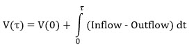
That is, the volume in the tank at any time in the future is equal to the initial volume plus the time integral of the inflow minus the outflow. If we further assume that the outflow (i.e., the leakage) is linearly proportional to the volume of water in the tank, the equation becomes:

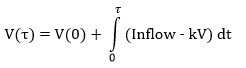
where k is the proportionality factor (i.e., the leakage fraction). Because the model itself is inherently a function of time (it is a time integral), we know that this model will display endogenous dynamic behavior. The key point is that the volume is not just a function of the instantaneous value of the inflow and outflow.  It is a function of all the past values of the inflow and the outflow. The model has “memory”.

Now let’s assume that the Inflow (and the leakage fraction) are constant (i.e., do not change with time).  In such a case, there are no exogenous factors controlling the dynamics. The result would look something like this:

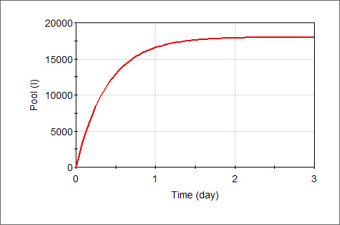
The tank volume increases until it reaches a steady state value. This is purely endogenous dynamic behavior. That is, the dynamic behavior is explained completely by the functional relationships of the model (i.e., the time integral).

Now let’s assume that the Inflow fluctuates with time.  The result would look something like this:

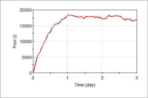
The dynamic behavior here is due to a combination of endogenous (the model structure) and exogenous (the inflow) factors. That’s what the real world looks like.