Lesson 3 - Representing Time in a Dynamic Simulation

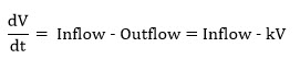
Systems that are changing with time are described mathematically using differential equations. In the example of the tank discussed in the last Lesson, we have the volume changing with respect to a single variable (time), so this can be described using an ordinary differential equation as follows:

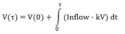
As shown in the previous Lesson, to write this in terms of the volume, we take the integral:

To solve for the volume as a function of time, we need to solve this integral. In simple systems (e.g., in this case, if the inflow was constant), we can solve this analytically. For almost any real system that you would be interested in modeling, however, an analytical solution is not available. Therefore, a dynamic simulator like GoldSim must solve such equations numerically (by computing an approximate solution).

To solve this (or any) integral numerically, it is necessary to discretize time into discrete intervals referred to as timesteps. GoldSim then “steps through time” by carrying out calculations every timestep, with the values at the current timestep computed as a function of the values at the previous timestep. In the case of the simple integral above, after discretizing time, GoldSim solves the equation by numerically approximating the integral as a sum:

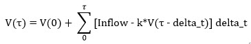
where delta_t is the timestep length.

Hence the volume at a particular time is computed based on the volume at the previous timestep. This particular numerical integration method is referred to as Euler integration. It is the simplest method for numerically solving such integrals.

The key assumption in the equation above is that the integrand (in this case the inflow and outflow) can be assumed to be constant over a timestep. The validity of this assumption is a function of the length of the timestep and the timescale over which the system is changing. The assumption is reasonable if the timestep is sufficiently small.

Hence, it is critical when carrying out a dynamic simulation that care be taken in selecting the timestep. In general terms, the appropriate timestep length is a function of how rapidly the system represented by your model is changing: the more rapidly it is changing, the shorter the timestep required to accurately model the system.

To get a feeling for the kinds of errors that can result from an inappropriate timestep when using Euler integration, let’s revisit the leaky tank model with some slightly modified inputs.  In particular, the Inflow will remain constant (we will not turn off the hose), and the tank leaks at a rate of 10%/hr.

As we pointed out above, if the inflow is constant, the integral describing that system can be solved analytically.  In the chart below, we show the analytical solution, along with various numerical solutions, each with a different timestep length (ranging from 0.03 days to 0.5 days):

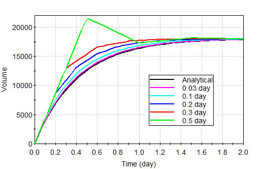
Note that with a very large timestep (0.5 days), the numerical solution is quite poor.  It gets progressively more accurate as the timestep gets smaller. With a timestep of 0.03 days, the numerical solution is, for practical purposes, indistinguishable from the analytical solution.

In this example, with all the timesteps used, the solution is stable (i.e., over time they all converge).  However, if the timestep is large enough, the solution actually becomes unstable (i.e., the solution does not converge and oscillates between large values).  It turns out that in this particular case, the stability requirement (which can be determined using a simple equation) is that the timestep be less than about 0.8 days (note that the accuracy of the solution becomes unacceptable well before the solution becomes unstable). 

So how do you select the proper timestep for a dynamic simulation? As a general rule, your timestep should be 3 to 10 times shorter than the timescale of the fastest process being simulated in your model. But what do we mean by the “timescale” of the process? In simple systems, you might be able to determine the timescales of the processes involved by inspection or a simple calculation. For example, in the example above, the outflow is controlled by the value of k (which is 10%/hr or 240%/day). We could roughly quantify the “timescale” of the process based on the “half-life” of the process (0.693/k).  In this case, it would be about 0.3 days. As can be seen, making sure the timestep is 3 to 10 times less than this results in an acceptable result.

In most models, however, it will likely be difficult to determine the timescales of all the processes involved. Therefore, after building your model, you should carry out the following experiment:

1. Carry out a simulation using your best guess as to the appropriate timestep.
2. Reduce the timestep length by half (increase the number of timesteps by a factor of 2), rerun the model, and compare results.
3. Continue to half the timestep length until the differences between successive simulations are insignificant.

Now that we have discussed timestepping conceptually, in the next Lesson we will see how you actually specify the various timestepping options in a GoldSim model.