Courses: Introduction to GoldSim:
Unit 7 - Modeling Material Flows
Lesson 13 - Managing Multiple (and Potentially Competing) Outflows from a Pool
As mentioned in the previous Lesson, if a Pool reaches its lower bound, the actual total outflow will be constrained (i.e., the total outflow cannot exceed the inflow, so it may be less than the sum of the requested outflows). Because a Pool has a separate output for each requested outflow, it provides a way for you to indicate that when the outflow is constrained, some of the outflows may have precedence over the others.
To illustrate this, let’s revisit the example we looked at in the previous Lesson. (Go to the “Examples” subfolder of the “Basic GoldSim Course” folder you should have downloaded and unzipped to your Desktop, and open a model file named Example2_SimplePool.gsm.)
Let’s take a closer look at this model. First, let’s open up Tank1 and go to the Outflows tab:
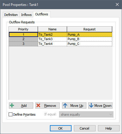
Each Outflow Request has a value (the Request) and a Name.
If you look at the three requests (represented using Data elements), you will see that they are as follows:
Pump_A = 20 l/min
Pump_B = 25 l/min
Pump_C = 15 l/min
So the total Outflow Request is 60 l/min.
There are two inflows: a constant inflow of 25 l/min, and a variable inflow that starts at 30 l/min but turns off after two days. Obviously, since the outflow requests are always greater than the inflows, eventually Tank1 will empty.
In fact, if you run the model and double-click on the Time History Result element named “Volumes”, you will see that Tank1 empties at about 2.7 days. After this point, there is still an outflow from the Pool (since there is still an inflow), but the total outflow is constrained to the inflow (which at 2.7 days is equal to 25 l/min).
Since the total Outflow Request is 60 l/min, obviously the various Outflow Requests must be constrained in some way to ensure that their total is equal to 25 l/min. How does GoldSim do that?
To answer that, take another look at the Outflows tab for Tank1. You should notice that this tab actually looks very similar to the dialog for an Allocator element that we discussed in Lesson 8. In particular, in addition to the Name and Request columns, there is another column called the Priority. This column is only used when the total outflow in constrained (i.e., the Pool is at its lower bound). When this happens, the element needs to allocate the actual outflow amongst the requested outflows. When the Pool is at the lower bound, the total outflow is constrained to be no greater than the inflow, so what is actually being allocated is the inflow.
By default, each Outflow Request has a fixed (and unique) Priority (which is an integer). The Priority of the Requests always decreases downward (with the first item having a Priority of 1). Priority 1 therefore represents the “highest” priority demand, 2 the next “highest”, and so on. To see how these Priorities affect the outflows, double-click on the Time History Result element named “Outflows from Tank1”:
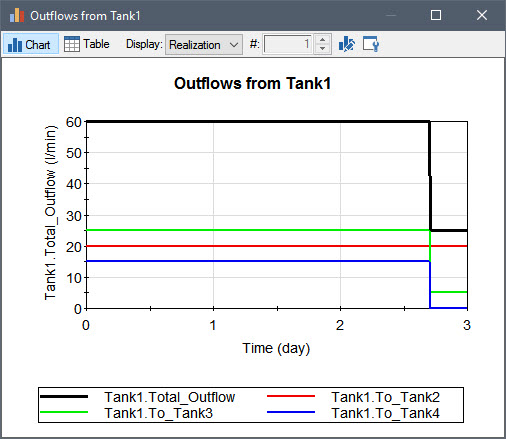
As can be seen, at about 2.7 days, the Total_Outflow drops from 60 l/min to 25 l/min (since the tank is empty and the total outflow is constrained to the inflow, which is 25 l/min). Of this 25 l/min, 20 l/min is allocated to Tank2, 5 l/min is allocated to Tank3 and none is allocated to Tank4. This occurs because the outflow to Tank2 has the highest (first) priority, so it receives all of it 20 l/min request. Tank3 has the next highest priority, but only receives 5 l/min (because that is all that is available). Tank4 receives nothing, since it has the lowest priority, and after Tank2 and Tank3, there is nothing left to allocate.
In this example, the three Outflow Requests had different Priorities. Let’s change that. Close the Result display, return to Edit Mode, and in the Outflows tab of Tank1, check the Define Priorities checkbox. The Priority column will become editable. Change all of the Priorities to 1. Now rerun the model and open the “Outflows from Tank1” Time History Result element again:
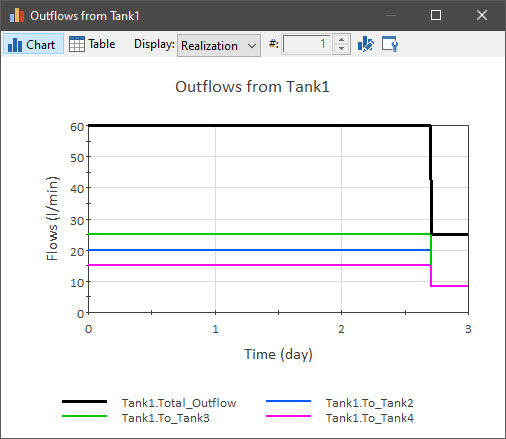
As can be seen, when the Total_Outflow drops from 60 l/min to 25 l/min at 2.7 days, the outflow is now shared equally (8.33 l/min) among the three Outflow Requests.
Note: If multiple outflows have the same Priority, you can specify the manner in which equal priorities are treated in the For equal priorities field. There are two options: 1) “share the input equally” (the default that was used in the example above); or 2) “share proportional to demands”. You can read about how GoldSim handles such in GoldSim Help.
These last two Lessons should make it clear why the Pool is a much more powerful element for modeling material flows than a Reservoir, as it effectively combines the features of the Sum, Allocator and Reservoir into a single element. As a result, as pointed out previously, going forward in this Course, we will use a Pool element exclusively for modeling material flows, and will no longer use a Reservoir.
Before leaving this Lesson, however, it is important to mention one additional topic associated with modeling competing outflows. In the example above, at the point in time that the total outflow became constrained, we immediately adjusted the outflows (e.g., in the case with equal priorities, all three were adjusted to 8.33 l/min).
If you think carefully about this, depending on the nature of the Outflow Requests, such a change may not always be physically realistic. In the case of this example, it would imply that the pumping rate could be changed (which, for example, would not be possible if the pumps were not variable speed).
In many cases, a more realistic representation is for the Outflows to be dynamically adjusted in response to the current Quantity. For example, as the Quantity decreases, some Outflows may decrease. Or perhaps, an Outflow is turned off prior to the Quantity hitting its lower bound. As we will discuss in detail in the next Unit, systems can be controlled in this way by using feedback loops.