Lesson 8 - Complex Dynamics Arising from Interacting Feedback Loops

We will model feedback loops again throughout the remainder of the Course. Before leaving the current discussion on topic of feedback loops, however, it is instructive to note that the interaction of multiple feedback loops can generate very complex endogenous behavior in a system, even in cases where the system appears to be conceptually simple.  A classic example of this can be illustrated by examining the population dynamics of predators and prey. In this Lesson we will explore an example model that illustrates complex dynamics (and widely different modes of behavior) arising from a relatively simple system.

The system we are going to consider is a simple model of deer and their predators (e.g., cougars).  This example is taken directly from Andrew Ford’s Modeling the Environment (2nd Edition), an excellent system dynamics text. If you are interested in exploring this example further, you can read about it in Chapter 20 of that text.

As mentioned above, we are going to consider a system consisting of two state variables (represented by Pools): the number of deer, and the number of predators.  In a more complex model, we could consider a larger number of Pools (e.g., by breaking the two species into different age groups and/or sexes).  But to keep the model simple, we will not do this.

We will also make the following simplifying assumptions:

• We are not representing any foraging limitations (the deer do not run out of food).
• The area where the species live is 800,000 acres in size. The system is “closed” in that neither predator nor prey can leave the area.
• We will assume an initial population of 4000 deer and 40 predators.
• The deer have a specified fractional net birth rate (births minus non-predator deaths) of 50%/yr.
• The rate of predation is a (non-linear) function of the density of deer.  As you can imagine, the more dense the population, the easier it is for predators to catch prey.
• The fractional birth rate for predators (%/yr) is a (non-linear) function of the predation rate.  The more deer that are caught, the higher the birth rate for the predators.
• The fractional death rate for predators (%/yr) is a (non-linear) function of the predation rate.  The more deer that are caught, the lower the death rate for the predators.

Rather than building this model, we are simply going to open and view a pre-built model. To do so, go to the “Examples” subfolder of the “Basic GoldSim Course” folder you should have downloaded and unzipped to your Desktop, and open a model file named Example4_PredatorPrey.gsm.  The model will look like this:

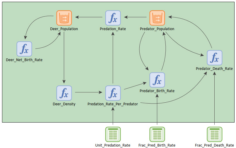
As you can see, this model is not terribly complicated. You are already familiar with all of the elements being used, and hence with a bit of effort should be able to explore the model and understand how it implements the assumptions listed above. The portion of the model in green represents the actual model structure.  The three Lookup Table elements at the bottom represent the key inputs (in particular, the three non-linear relationships mentioned above).

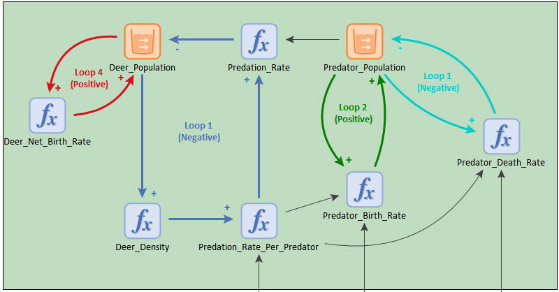
So how many feedback loops does this model have?  Believe it or not, it actually has six! Four of these are quite obvious and are highlighted below:

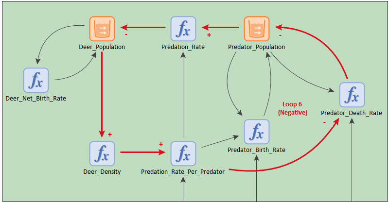
Two additional loops are shown below:

As you might expect, given that this structure actually has six feedback loops, it can generate some very complex behavior. In fact, it turns out that the behavior of the model can change drastically based on the input assumptions.

Let’s run the model and look at some results.  Run the model and double-click on the Time History Results element named “Results”:

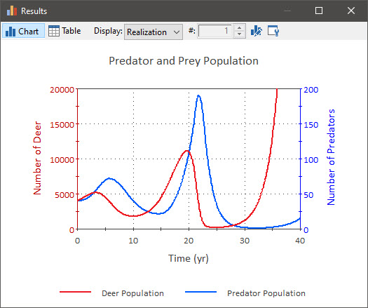
For this set of inputs, what we see is that after some growing oscillations, both populations crash and become extinct. (There actually appears to be a mathematical rebound after the crash, but in reality, populations cannot survive when their numbers fall below a minimum viable number, and this particular fact is not represented in the model). This unstable mode of behavior can be referred to as “growing oscillations/extermination”.

It turns out that in the real world, predators do not normally drive prey to extinction.  Among other things, as the prey density gets smaller, it becomes easier for the prey to hide, and they become significantly harder to catch. This relationship is represented in the Lookup Table named Unit_Predation_Rate.  This Lookup Table describes the predation rate as a function of the prey density.  The function we used in this model is plotted in the figure below as “Base Case”.

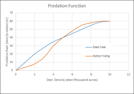
“Better Hiding” represents a modified function in which we have changed the function so that the predation rate becomes smaller at low prey density.

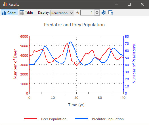
This new function has been implemented in the model file named Example5_PredatorPrey.gsm in the “Examples” subfolder of the “Basic GoldSim Course” folder you should have downloaded and unzipped to your Desktop (that is the only difference between the two models).  If you open that model, run it and look at the results, they look like this:

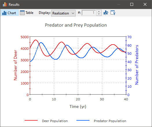
By simply changing the predation function slightly, we see that we no longer have unstable behavior.  Instead, what we see is cyclical behavior with a period of about 10 years.  There is a two year lag between the peak of the deer population and the peak of the predator population. 

In this particular case, the cycles are actually damped (the amplitudes are decreasing), so that if we ran this model long enough it would reach a dynamic equilibrium with 4000 deer and 50 predators. (If you are interested, rerun the model with a Duration of 200 years to see this.) This stable mode of behavior can be referred to as “damped oscillations”.

Let’s add one more minor modification to the model to make it a bit more realistic.  As we will discuss in great detail in Unit 11, random variations in inputs can often have important impacts on model behavior.  We are going to show how a simple random variation in the deer net birth rate can greatly affect the behavior of the model.  In the previous two models you have looked at, we have assumed that the deer population increases at a rate of 50%/yr (this accounts for new births and deaths not associated with predation). In our final example model, we are going to assume that this rate varies randomly, ranging from 30%/yr to 70%/yr.  It changes randomly every year (i.e., the value is resampled once per year) to represent “good years” and “bad years” (e.g., due to weather and food availability) that are not otherwise represented by the model (i.e., this is an exogenous factor).

This new net birth rate has been implemented in the model file named Example6_PredatorPrey.gsm in the “Examples” subfolder of the “Basic GoldSim Course” folder you should have downloaded and unzipped to your Desktop (that is the only difference between this and Example5_PredatorPrey.gsm).  If you open that model, you will see a new element (a Stochastic):

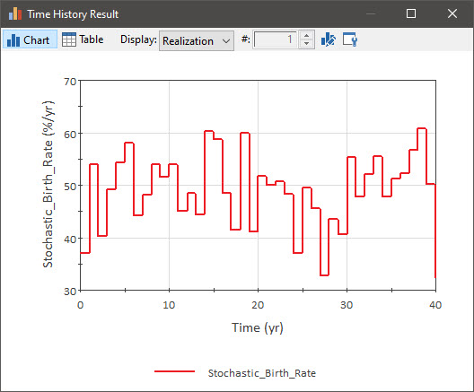
This is the element that implements the random behavior.  Don’t worry about how this element actually does this for now (we will discuss it in detail later in the Course).  It is sufficient to simply plot this value to see what it does.  Run the model and right-click on the Stochastic_Birth_Rate element and plot its time history.  What you will see is that the fractional birth rate randomly varies from year to year:

If we now look at the Result element, we see the following behavior:

What is interesting here is that the oscillations, although they are much more irregular, no longer appear to be damped.  (You can confirm this by running the model for 200 years). What actually is happening is that each year the system is disturbed (and hence can be thought to be “reset”).  As a result, the system never has a chance to be fully damped. This illustrates that randomness can change a damped system into one with oscillations that continue indefinitely. This stable mode of behavior can be referred to as “damped oscillations that are sustained through disturbance”.  Interestingly, in real world predator-prey systems among mammals it is not uncommon to see sustained (but somewhat irregular) 9 to 10 year cycles like this.

Of course, we have simplified this system in a number of ways.  We could have considered a larger number of Pools (e.g., by adding forage material, by breaking the two species into different age groups and/or sexes).  We also could have added more feedback loops (e.g., by adding a Pool representing the amount of forage material for the deer and how the deer population modifies this). However, the purpose of this Lesson was not to teach you about predator-prey systems.  Rather, it was simply to use an interesting example to illustrate that the interaction of multiple feedback loops can generate very complex behavior in a system, even in cases where the system appears to be conceptually simple.