Lesson 2 - Understanding Feedback Loops

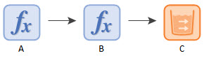
Simple models have a direct chain of causality: input data affect some elements, which affect other elements, and so on, until eventually the elements which calculate the desired results of the model are reached:

More realistic systems, however, contain elements whose output can, directly or indirectly, affect one of their own inputs. This creates a looping or circular system structure, such as this:

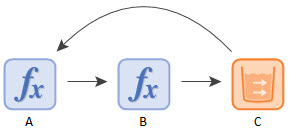
This particular structure represents a feedback loop. As we mentioned in the previous Lesson, feedback loops are present in one form or another in most real-world systems, and can be readily modeled in GoldSim. In the example above, A affects B which affects C, and then C “feeds back” to affect A and so on. That is, feedback loops represent a looping chain of cause and effect. Note that the terms “feedback” and “cause and effect” intentionally imply that the relationship between the variables is dynamic and the system changes over time (although as we shall see in a subsequent Lesson, systems with feedback loops can also reach a dynamic equilibrium).

There are two kinds of feedback loops: positive feedback loops and negative feedback loops.

• Positive feedback loops are self-reinforcing. Positive feedback loops generate growth and amplify changes. The more adult rabbits you have, the more baby rabbits that are produced; the more baby rabbits that are produced, the more adult rabbits you have, and so on until the world is full of rabbits (or this positive loop is counteracted by one or more negative feedback loops).
• Negative feedback loops are self-correcting. Negative feedback loops drive systems toward equilibrium and balance. The more rabbits you have, the less food you have; the less food you have, the higher the death rate of rabbits (and hence the less rabbits you have).

The dynamics of most systems are driven by the interactions of many such loops. Different combinations of such loops (and delays) can be shown to produce various fundamental modes of dynamic behavior (e.g., exponential growth, goal-seeking, oscillation). There is a very well-developed and extensive academic literature surrounding the methodology and modeling techniques for analyzing and understanding the behavior of systems governed by such loops (and delays) referred to as system dynamics.

The system dynamics methodology uses causal loop diagrams as a visual tool to represent the feedback structure of systems. For example, the causal loop diagram for the two loops mentioned above would look like this:

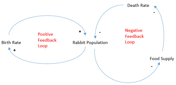
Each arrow indicates a cause and effect link between variables and has a “+” or “-“ sign. A positive link between variables indicates that if the cause (e.g., Rabbit Population) increases, the effect (e.g., Birth Rate) increases (and, conversely, as the cause decreases, the effect decreases). A negative link between variables indicates that if the cause (e.g., Rabbit Population) increases, the effect (e.g., Food Supply) decreases (and, conversely, as the cause decreases, the effect increases). It can be shown that if the number of negative links in a loop is even, the loop is a positive feedback loop; if the number of negative links in a loop is odd, the loop is a negative feedback loop. So in this simple system, we see that the loop on the left is a positive loop: if the rabbit population increases, the birth rate increases, which increases the rabbit population. This generates growth. The loop on the right is a negative loop: if the rabbit population increases, the food supply decreases; if the food supply decreases the death rate increases; if the death rate increases, the rabbit population decreases. This acts as a “check” or balance on the population growth. These two loops interact, and depending on the parameters describing the rates, they could result in different modes of behavior.

Of course, this is a simplified system.  We could add more loops to make it more realistic.  For example, you can imagine that predators could interact with the rabbit population, affecting the rabbit death rate (and the rabbit population, as it changes, could in turn impact the predator birth and/or death rate).  It is also worth noting that there are likely to be delays in some loops. For example, decreasing the food supply might not immediately increase the death rate.  It would likely take some time for this to have an impact. These features would add to the dynamic complexity of the system.

Although diagrams like this can be useful when trying to understand the general behavior of some kinds of systems (and the system dynamics community puts great emphasis on them), they are not required in order to build a model (if you are interested in learning more about these diagrams, refer to the Ford book mentioned above). The point here is just to get you to start to think about and understand feedback loops, as they will be present in almost any system you will want to simulate. In later Lessons in this Unit, we will build or examine several different systems incorporating such feedback loops.