Lesson 7 - Controlling Mass Transfer through Diffusive Barriers

The Exercise that we worked through in the last Lesson was actually fairly realistic. That is, diffusive engineered barriers (in the form or caps, covers or surrounding material) are often used to control the release of contaminants.  This can be seen for systems like the one we considered in the previous Lesson (covering contaminated materials at the bottom of a water body) or for controlling the release of chemicals from soils or other materials near the ground surface. For radioactive waste management applications, a diffusive barrier (e.g., of bentonite surrounding waste containers) often acts a major component of engineered barrier systems designed to slow the release of radionuclides for disposed containers.

In the previous Lesson, we noted how our diffusive sediment barrier reduced the pond concentration.  Could we reduce the concentration in the pond further?  It turns out that we could in fact do this by limiting the diffusive mass transfer rate (e.g., by selecting a material with a smaller porosity and/or tortuosity). If the contaminant itself had a lower diffusivity (something we cannot control), the pond concentration would also be reduced. This is not unexpected, since as discussed in Lesson 3, the diffusive mass transfer rate is proportional to the diffusive conductance (τ n D_m A / Δx).

Moreover, in most situations, engineered diffusive barriers do not just depend on the porous medium slowing the diffusion process physically.  They also often involve use of porous media that act to slow the diffusion process chemically (due to partitioning).  That is, they sorb the contaminants as they diffuse through the material.  This can have a very significant impact on the performance of the diffusive barrier.

To understand conceptually why this is the case, recall from Unit 3, Lesson 5 that by assuming equilibrium partitioning with a single solid, we can express the concentration of a species in water within a porous medium in some fixed volume (e.g., a well-mixed Cell) as:

where V represents the volume of water (e.g., within one of our slices), G represents the mass of solid, and K is an equilibrium partition coefficient that describes the ratio of the concentration on the solid to the concentration in the water at equilibrium. Hence, partitioning affects the concentration of the diffusing contaminant (reducing it), and this in turn affects the concentration gradient (in a discretized model, the concentration difference between two Cells). This acts to slow diffusion.  As we will see, however, its effects are not exactly the same as reducing the diffusive conductance (e.g., by reducing the tortuosity, porosity or diffusion coefficient).

To get an idea of the effect of the diffusive conductance and partitioning on diffusion through a porous medium, let’s first revisit the tube example we explored in Lesson 5. Go to the “Examples” subfolder of the “Contaminant Transport Course” folder you should have downloaded and unzipped to your Desktop, and open a model file named ExampleCT20_Diffusive_Tube_Retardation.gsm.

This model is identical to the diffusive tube model we looked at previously with the following changes:

• Two additional species have been added (Y and Z).
• Species Y has a partition coefficient equal to 1.875E-04 m3/kg (X and Z have zero partition coefficients). This is done by defining Partition Coefficients for the Sand.
• Species Z has a diffusivity that is half that of X and Y. This is done by defining Relative Diffusivities for Water.

You are encouraged to browse the model to understand these changes. Run the model and go to the Tube Container.  Let’s first look at the concentration of the three species in the last Cell (Cell10).  There is a Time History Result element named “Concentration 10” set up to look at this:

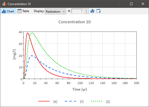
X represents the species with the original diffusion coefficient (and no partitioning).  What we are interested in evaluating is how adding sorption (Y) or decreasing the diffusive conductance (Z) changes the behavior. What we see is that in both cases, the time it takes the mass to diffuse out of the system is longer.  In fact, we can quantify the degree to which the rate of diffusion has been reduced.  First, let’s look at when the peak concentration occurs.  We could do this by just looking at the chart.  But we can also set up an Extrema element that records the time of the peak value.  That has been done in this model, and the result is displayed (in table form) in the Array Result element named “Time of Peak”:

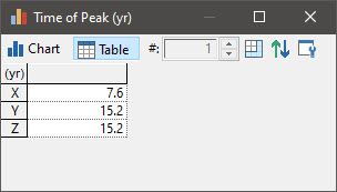
As can be seen, the peaks of Y and Z and delayed by exactly a factor of two. 

Another way to quantify the delay is to look at when 50% of the mass has diffused through the column.  The “Cumulative Release” Time History Result element displays this:

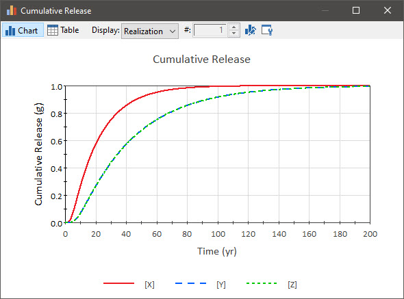
If you go to a table view and look for the point at which the value is equal to 0.5 g, you will find that X reaches this value at between 17.1 years and 17.2 years, and Y and Z reach this value at 34.3 yrs (exactly twice the time).

It is not surprising that Z moved two times slower through the tube (since we reduced its diffusive conductance - by changing the diffusion coefficient - by a factor of two).  But why did Y move exactly two times slower?  It did so because the partition coefficient was selected to produce this result. The delay or slowing of a species due to partitioning can be quantified in terms of a retardation factor:

The retardation factor is most commonly used when discussing advective-dispersive transport (and we will do so in the next Unit), but it can also be applied for diffusive transport. In this example, if you substitute the various values into this equation you will find it has value of 2.

Note that although reducing the diffusive conductance and adding a retardation factor both delayed the diffusive rate by a factor of two, their impact on the concentration in the last Cell was not identical. In fact, you can see that at any given time the concentration of Y is half of that of Z (due to the partitioning).

The “Rate” Time History Result displays the diffusive mass transfer rate out of Cell10:

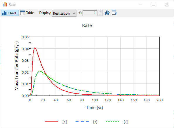
As we can see, Y and Z are identical (and exactly half the value of X).  That is, although the concentration in Cell10 is different for Y and Z, the mass transfer rate out of the tube is identical.  This is because the mass transfer rate is simply (diffusive conductance) * (Cell10 concentration – Tank concentration).  The Tank concentration is fixed at zero.  Cell10 concentration for Z was twice that of Y, but the diffusive conductance for Z was half that of Y (due to the change in the diffusion coefficient).  So both act to slow diffusion, but in two different ways: one reduced the diffusive conductance and one reduced the concentration gradient.

In this example, these two mechanisms produced the same diffusive mass transfer rate out of the system, but that is not always the case.  To see this, let’s now first revisit the sediment example we explored in the previous Lesson. Go to the “Examples” subfolder of the “Contaminant Transport Course” folder you should have downloaded and unzipped to your Desktop, and open a model file named ExampleCT21_Sediment_Diffusion_Kd.gsm.

This model is identical to the diffusive sediment model that you built with the following changes (similar to the changes we made for the tube model):

• Two additional species have been added (Y and Z).
• Species Y has a partition coefficient equal to 1.4E-04 m3/kg (X and Z have zero partition coefficients). This is done by defining Partition Coefficients for the Sand.
• Species Z has a diffusivity that is half that of X and Y. This is done by defining Relative Diffusivities for Water.
• The model is run for 50 years (instead of 40 years).

You are encouraged to browse the model to understand these changes. Note that this partition coefficient was selected to result in a retardation factor for Y of 2.

It is important to recall that conceptually this model is very different from the tube model. In the tube model a slug of mass diffused through the system (and eventually all mass diffused out of the system). In this model, we are assuming an effectively “infinite source”, such that the system reaches some steady state. As such, there is always mass in the pond (it is never completely flushed due to the infinite source).  In this model, our goal is twofold: 1) to reduce the steady state concentration; and 2) to delay the time to reach steady state (we will discuss why this can be critical shortly).

In this regard, this model is actually more representative of the type of problems you would likely need to model in the real world (having such an infinite source due, for example, to the slow dissolution of a large mass of waste, is not unusual). Moreover, you will see that because they act via different mechanisms, the effects of retardation and diffusive conductance on behavior are different than what we saw for the tube model.  

Run the model and go to the Cells Container.  Let’s first look at the concentration of the three species in Sediment5 (the top layer of sediments closest to the pond water).  There is a Time History Result element named “Concentration in Sediment5” set up to look at this:

What we see here is that both Y and Z are delayed (they reach 50% breakthrough and steady state two times later than X).  But we find that all three steady state concentrations are identical.

So what is happening here? The mass transfer rate through the sediments (e.g., between any two sediment Cells) is equal to the (diffusive conductance) * (concentration difference).  The concentration difference between any two sediment Cells initially changes with time, but eventually reaches some steady state value.  And at steady state, for any two Cells, these differences must be nearly identical for all three cases. This is because the overall concentration gradient through the sediments is ultimately (at steady state) controlled by two end points: the contaminated layer, which is fixed at 100 mg/l, and the pond, which is flushed relatively rapidly, so that it has an insignificant value relative to the contaminated layer (as we will see, it differs for the three species, but is always much less than 100 mg/l).  As a result, the concentration at the top of the sediment layer must eventually be the same in all three cases, as the gradient across the sediments is eventually identical in all three cases.

Now let’s look at the concentration in the Pond (there is a Time History Result element named “Pond Concentration” set up to look at this):

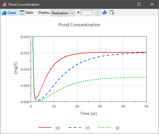
Here we see that the partition coefficient has no impact on the steady state pond concentration, but the reduced diffusive conductance does.  Why is this the case?  As we pointed out above, the steady state concentration in the last sediment layer is identical (and much higher than the pond concentration) for all three cases.  As a result, the concentration difference between Sediment5 and Pond is the same in all three cases. But the diffusive conductance for Z is half that of X and Y.  As a result, the mass transfer rate from Sediment5 to the Pond for Z is half that of X and Y. This results in a pond concentration that is 50% lower.

So for this type of model (in which we have an “infinite source” of a contaminant that must then diffuse through a diffusive barrier and into a low concentration region), we can conclude the following:

• Decreasing the diffusive conductance (we did this by decreasing the diffusivity, but practically you would do this by selecting a porous medium with a lower porosity and tortuosity) has the effect of delaying the time to reach steady state as well as reducing the steady state mass transfer rate out of the barrier (and steady state pond concentration).
• Increasing the retardation factor (by selecting a porous medium which sorbs the contaminant) has the impact of delaying the time to reach steady state, but does not change the steady state mass transfer rate out of the barrier or the pond concentration.

This, however, is for a species that does not decay. If a species decays (and does not ingrow), it could decay to a large extent before it has a chance to exit the diffusive barrier. In fact, for applications in which the contaminants are decaying (e.g., radioactive waste management applications), delaying the breakthrough via sorption may be one of the primary objectives of the diffusive barrier.