Unit 8 - Representing Complex Dynamics: Loops and Delays

Lesson 7 - Simulating Feedback Control

In the previous two Exercises, we played with a simple example of how feedback can control the behavior of real-world systems. In those Exercises, the feedback involved a passive, natural process (evaporation). That is, the process occurred naturally and we didn’t really have much active control over it. In many engineered (and social and organizational) systems, however, there is active feedback control designed directly into the system to make it behave in a specified manner. A thermostat is the classic example of this (the heating and/or cooling rate is adjusted based on the current temperature).

You should recall that we mentioned this issue in Unit 7, Lesson 13 when we discussed how a Pool manages multiple and competing outflows as it approaches its lower bound (and the outflow becomes constrained). We pointed out that in many cases, competing outflows actually need to be dynamically adjusted in response to the current Quantity. For example, as the Quantity decreases, some Outflows may decrease (this could be a passive or active process). Or perhaps, an Outflow is actively turned off prior to the Quantity hitting its lower bound.

If you are going to model such systems, you need to understand how to properly represent these controlling feedback loops in a realistic way. If the inflow or outflow is adjusted smoothly in response to the change in the Quantity (as was the case in the previous Exercise illustrating a passive feedback control system), there is typically no problem. But many active feedback control systems require inflows and outflows to be “turned off” or “turned on” suddenly when a particular Quantity is reached (a thermostat is an example). In these cases, it is quite common for novice (and even some experienced) modelers to represent such systems in such a way that the model behaves quite poorly (e.g., oscillates unrealistically).

The goal of a feedback control system is generally to control the value of a state variable (defined in Lesson 3) in the system by actively adjusting additions (inflows) to and withdrawals (outflows) from that variable. In the case of the thermostat, the state variable is the amount of heat in the house (quantified via the temperature) and the additions and withdrawals are controlled by turning on/off the heat or air conditioning. For a pond, the state variable is the amount of water in the pond (which could be quantified via a water level) and some inflows and outflows are controlled by turning on/off pumps that remove (or perhaps add) water.

To briefly illustrate the basic concept of active feedback control, let’s consider a very simple problem: water flows into a pond (in which we have no control over that inflow), and we wish to actively control the volume of water in the pond by turning a pump (that removes water from the pond) on and off in a specified manner. Rather than building this model, we are simply going to open and view a pre-built model. To do so, go to the “Examples” subfolder of the “Basic GoldSim Course” folder you should have downloaded and unzipped to your Desktop, and open a model file named Example3_Feedback_Control.gsm. The model will look like this:

Examine this model and you will see that it is quite simple. There is an Initial Volume (1 m3), a constant Inflow to the pond (100 m3/day), and a Target volume (300 m3). The Withdrawal (outflow) from the pond is the following Expression:

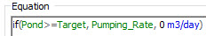
That is, when the pond volume is greater than or equal to the target volume, the pump is turned on. When it is below the target volume, it is turned off. Note that the Pumping_Rate is larger than the Inflow (it is defined as 200 m3/day), so when the pump is turned on, the volume in the pond is reduced. The feedback loop between the Pond and the Withdrawal is apparent.

So will this logic work? At first glance, it seems to make sense, but if you run the model and look at the results, you will quickly realize that a real system would be unlikely to be controlled by logic like this. Run the model and double-click on the Time History Result element. The result looks like this:

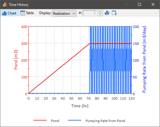
As you can see, the pond fills up, and the volume does remain very close to 300 m3. However, if we look at the pumping rate, we see that we have created a system that oscillates rapidly. As soon as the volume reaches the target, the pump turns on, the volume is reduced and the pump turns off, and so on. The timestep for this model is 1 hour, and hence the pump oscillates on and off every hour. In fact, if we reduced the timestep to 1 minute, as long as the pumping rate is high enough (and it is), it would oscillate every minute! If the Initial Volume starts above the target rather than below, you would also see this same oscillatory behavior once it reached the target. Clearly, the system would never be designed to operate like this in the real world. If a thermostat worked this way, the furnace would be turning on and off every few seconds!

In this example, the goal is to control the state variable (e.g., volume) around a particular “target” level. Although this is a common objective (e.g., a thermostat does this), it is also quite common for feedback control systems to be used to control the behavior of a system as it approaches its bounds (e.g., controlling the pumping rate to or from a pond as it approaches its upper limit or as it empties). In this case, you can imagine the need to actively adjust flows as the volume approaches the bounds.

Note: Unfortunately, when using poorly designed feedback logic (such as the logic outlined above), if the target is near or at the Upper or Lower Bound for the Pool (particularly if multiple Pools are involved), the model can often oscillate even more rapidly. This is because as discussed previously (Unit 7, Lesson 4), GoldSim inserts unscheduled updates whenever a bound is reached (that section discussed a Reservoir; but the same thing applies for a Pool). Poorly designed feedback logic could result in the state variable continuously oscillating at the bound (with a timestep being inserted each time the bound is reached). This can result in timesteps being inserted practically continuously (e.g., every second or less)!

So, the simple example we have shown here, although at first glance seemingly correct, clearly is incorrect and results in unrealistic behavior. Unfortunately, it is quite common to find models that are structured like this. Can we do better? Absolutely. In fact, it is possible to model such a system very realistically and efficiently (with no unrealistic oscillations at all). However, in order to do so, we will require use of a GoldSim element we have not yet discussed. So we will revisit this problem later in the Course.

For now, it is sufficient to understand that active feedback control loops are an important component of many engineered (and organizational) systems, and it is critical to have a good understanding of how the real system works, such that what you represent is realistic (i.e., it represents something that could be practically implemented in the real world). We will discuss how to represent such systems in a realistic way in Unit 13.