Lesson 4 - Exercise: Modeling an Evaporating Pond

In the previous Lesson, we quickly built a simple model that involved a feedback loop.  In this Lesson we will carry out an Exercise that builds a slightly more complicated model that we will examine more closely, and build upon over several subsequent Exercises.

We are going to simulate a pond that fills with water. However, water also continuously evaporates.  This model is similar in many respects to the first model we built in Unit 4 (the leaky tank being filled with a hose), so it should be very easy for you to build.

We are going to create a new model, and will assume the following:

• The pond is initially empty.
• There is a constant inflow to the pond of 10 m3/day.
• We will assume that the pond’s capacity is so large that we don’t need to specify an Upper Bound (as we won’t reach it).
• The pond evaporates at a rate that is linearly proportional to the volume of water in the pond.  In particular, 6% of the pond volume evaporates per day.

We want to calculate the volume of water in the pond over the next 100 days.

So to create this model, you will need to create two Data elements (for the inflow and the evaporation fraction), an Expression (for the actual evaporation rate), and a Pool element to represent the pond. In particular, you should do something like this:

• Create a Data element named “Inflow”. The Display Units should be specified as m3/day. Define it as 10 m3/day.
• Create a Data element named “Evaporation_Fraction”. The Display Units should be specified as %/day. Define it as 6 %/day.
• Create a Pool named “Pond” with Quantity Units of m3 and Flow Units of m3/day. Add an Inflow linked to the “Inflow” Data element.
• Create an Expression named “Evaporation” with Display Units of m3/day.  Define it as “Pond * Evaporation_Fraction”.
• Edit the Pool and specify the single Outflow Request as “Evaporation”.
• Create a Result element (named “Results”) that plots the pond volume.

We will run the model for 100 days with a 1 day timestep.

Stop now and try to build and run the model.

Once you are done with your model, save it to the “MyModels” subfolder of the “Basic GoldSim Course” folder on your desktop (call it Exercise7.gsm). If, and only if, you get stuck, open and look at the worked out Exercise (Exercise7_Evaporating_Pond.gsm in the “Exercises” subfolder) to help you finish the model.

Your model structure should look something like this:

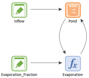
As noted previously, when you first create the model, it will look like there is a double-headed arrow (influence) between Pond and Evaporation.  Actually, this is not a double-headed influence at all.  There are actually two influences sitting right on top of each other. If you left-click on the double-headed arrow, a point will appear in the middle. You can then select it (by left-clicking) and drag it (while holding the left mouse button down).  You will then see that there are in fact two influences.  You can drag the other one in the opposite direction to make it look like the image shown above.

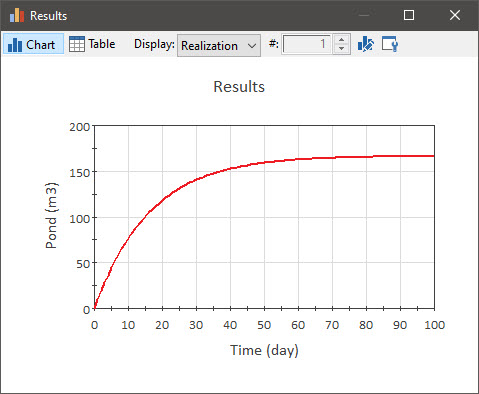
The result for the Pond should look like this:

Based on our previous discussions, it should be clear that this model has a feedback loop. Moreover, you should be able to discern that this is a negative feedback loop.  Why? First, let’s quickly look at the causal loop diagram for this:

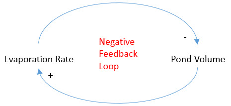
As we can see, as the pond volume increases, the evaporation rate increases; but as the evaporation rate increases, the pond volume decreases. This is a negative feedback loop (an odd number of negative links).

The plotted result also indicates that this is a negative feedback loop.  Negative feedback loops drive systems toward equilibrium and balance. In this case, the system reaches a dynamic equilibrium (in which the evaporation rate increases until it balances the inflow rate).