Lesson 2 - Basic Simulation Concepts

The term simulation is used in different ways by different people. As used here, simulation is defined as the process of creating a model (i.e., an abstract representation or facsimile) of an existing or proposed system (e.g., a business, a project, an organization, a facility, an ecosystem, a lake, a machine) in order to identify and understand those factors which control the system and/or to predict (forecast) the future behavior of the system.

Almost any system that can be quantitatively described using equations and/or rules can be simulated.

Although certain types of simulations can be static (i.e., the system is assumed not to change with time), most simulations of interest are dynamic.

In a dynamic simulation, the system changes and evolves with time (in response to both external and internal influences), and your objective in modeling such a system is to understand the way in which it is likely to evolve,  predict (forecast) the future behavior of the system, and determine what you can do to influence that future behavior. That is, the purpose of a dynamic simulation is typically to predict the way in which the system will evolve and respond to its surroundings, so that you can identify any necessary changes that will help make the system perform the way that you want it to.

For example, you could dynamically simulate (predict) the amount of money in your bank account over the next year in order to quantitatively understand the impacts of possible actions (e.g., changing jobs, modifying spending habits) to ensure that your balance does not go negative at some point in the future. To build such a model, you would need to quantitatively describe things such as how often you get paid, how much you receive each paycheck, what your various monthly expenses are, etc. The key output of such a simulation might look like this:

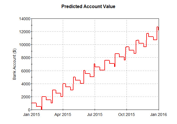
This chart (referred to as a time history) shows how the amount in the bank account is predicted to change over time.

The chart above is the output of a deterministic simulation. A deterministic simulation represents parameters, processes, and events using specified (“known”) values, perhaps described as "the best guess", “typical”, “best case” or "worst case" values. The result of running several deterministic simulations (e.g., best guess, optimistic inputs, pessimistic inputs) is a qualitative statement such as this:

"It is possible under some circumstances or scenarios that my account balance may go negative over the next year."

Such a statement is of limited value due to its qualitative nature. What you really would want to know is the likelihood of your account going negative.

To do so, you would need to account for the uncertainty in the key inputs in the model (e.g., your spending habits, unexpected expenses, etc.). Probabilistic simulation represents such uncertainty explicitly and quantitatively. If an input is uncertain, it is defined using a probability distribution. If the inputs to a model are uncertain, the outputs are necessarily uncertain.  Within GoldSim, the uncertainty in inputs is propagated to the uncertainty in the outputs using a technique known as Monte Carlo simulation. In Monte Carlo simulation, the entire system is simulated a large number (e.g., 1000) of times. Each of these simulations is referred to as a realization of the system, and represents a possible future (i.e., one possible path the system may follow through time). Here is a chart showing 10 different realizations (10 equally likely possible futures) of the bank account value, explicitly accounting for uncertainty in the inputs:

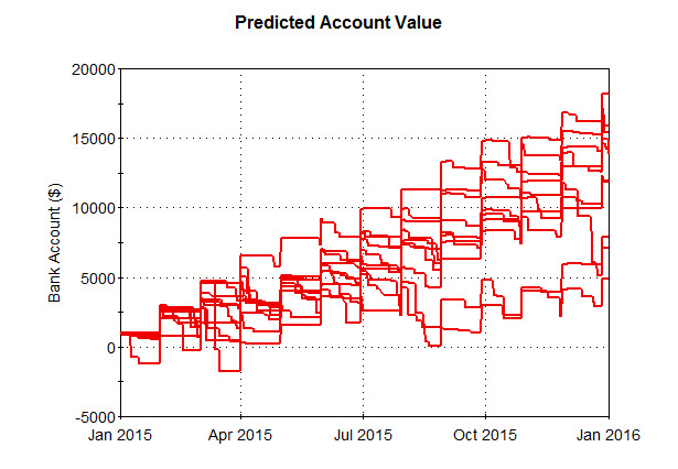
The 10 realizations are different due to the uncertainty in the input values (e.g., spending habits). The various realizations can subsequently be assembled into an output probability distribution. (This expresses the idea that if the inputs are uncertain, the outputs are uncertain).

The chart below shows the output of a probabilistic simulation of a large number of realizations (in which the uncertainty in spending habits is explicitly represented):

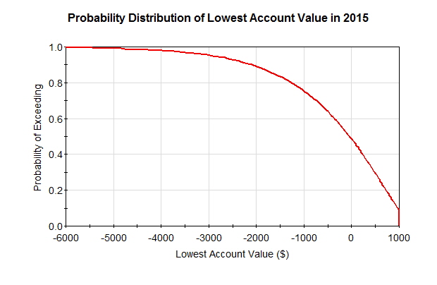
This chart displays the lowest account balance ever encountered during the simulation (i.e., over the entire year) as a probability distribution. This particular type of probability distribution display is referred to as a CCDF, and we will discuss it in detail in a subsequent Lesson.  However, it is quite simple to describe and understand.  The y-axis shows the probability of exceeding the value on the x-axis.  So in this case, if we go to $0, we see there is about a 50% chance that the lowest account balance will always be above $0 (and hence a 50% chance it will become negative at some point).

Hence, the result of a probabilistic simulation of a system is a quantified probability such as this:

"There is about a 50% chance that my account balance will go negative over the next year."

A quantitative statement such as this is much more useful than a simple qualitative statement.

In particular, given the predicted result above (a significant probability of an outcome you would want to avoid), you might then choose to modify your spending habits (or find a better paying job)!  Moreover, with a simulation model, you could assume some change in your behavior or situation (e.g., different spending habits, higher salary), rerun the model, and see how the change would affect the likelihood that your account value will go negative.

Throughout this Course we will explain and discuss all of the simulation concepts mentioned above in great detail. For now, however, it is sufficient to note that, as this simple example illustrates, simulation is a powerful and important tool because it provides a way in which alternative designs, plans and/or policies can be evaluated without having to experiment on a real system, which may be prohibitively costly, time-consuming, or simply impractical to do. That is, it allows you to ask “What if?” questions about a system without having to experiment on the actual system itself.