Lesson 7 - Running a Model and Viewing Results

In order to simulate how a system might evolve over time in a program like GoldSim, it is necessary to discretize time into intervals of time referred to as timesteps. We will discuss this in detail in a later Unit, but for now it is sufficient to note that GoldSim “runs the model” by “stepping through time”, carrying out calculations every timestep, with the values at the current timestep often computed as a function of the values at the previous timestep.

Hence, in order to dynamically simulate a system in GoldSim, you must specify the duration of the simulation (e.g., 1 year) and the length of the timestep (e.g., 1 day). The appropriate timestep length is a function of how rapidly the system represented by your model is changing: the more rapidly it is changing, the shorter the timestep required to accurately model the system (and as we will see in a later Unit, the timestep does not necessarily have to be constant).

If you are running a probabilistic simulation, you must also specify how many realizations of the model you would like to run.  Recall from Lesson 2 of this Unit that a realization represents a possible “future” for an uncertain system (i.e., one possible path the system may follow through time) and that running multiple realizations of a model is referred to as Monte Carlo simulation.

After running a model, GoldSim can generate and display different types of results, in either graphical or tabular form. The most common results viewed are time history results and distribution results.

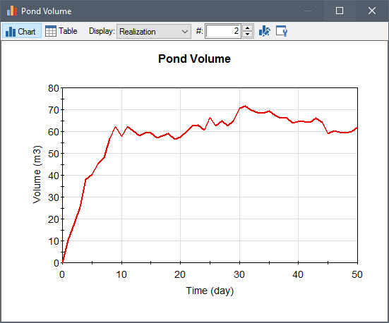
A time history result simply shows how a model output is predicted to change with time. As such, it is the fundamental type of result produced by a dynamic simulation model.  The x-axis is time (or dates) and the y-axis is the value of the output. An example of a simple time history is shown below:

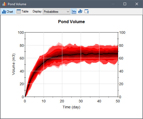
A probabilistic time history result (showing percentile bands) displays the range of outcomes that an output may have, accounting for the uncertainty in the model inputs.  It looks like this:

A distribution result is the fundamental type of result produced by a probabilistic simulation model. A distribution result shows a probability distribution of an output at a specific point in time (e.g., the end of the simulation): 

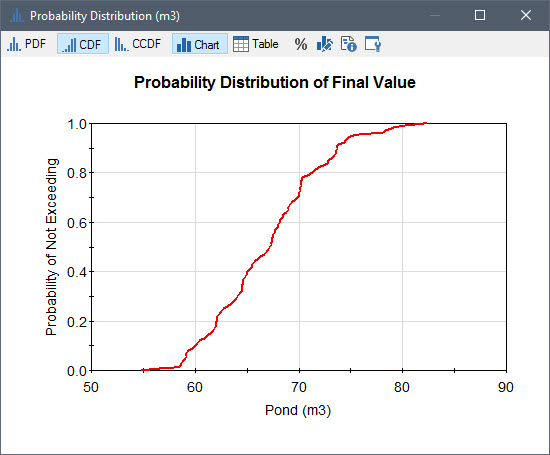
The particular type of chart shown above, referred to as a CDF, is the complement of a CCDF (discussed previously in Lesson 2 of this Unit).  The y-axis shows the probability of not exceeding the value on the x-axis.  So in this example, if we look at an x-axis value of 60 m3, we see there is about a 10% chance that volume at the end of the simulation will not exceed that value (and hence a 90% chance that it will exceed that value).