Lesson 3 - Physical Processes Controlling Mass Transport: Advection

The cornerstone of any mass transport model is the concept of mass balance or mass conservation. As we have noted, when mass transport equations are solved, it is necessary to discretize space into discrete volumes or compartments. Mass is spread out equally throughout any particular discretized volume instantaneously (i.e., the volume is instantaneously well-mixed). For each such compartment in the model (and for each chemical or contaminant being considered) the mass balance equation takes the following form:

(Rate of change of mass) = (mass transport in) – (mass transport out) + (mass production internally) – (mass elimination internally)

To discuss the various processes in this and the next several Lessons, we will consider this equation for some very simple examples.

Let’s first consider two tanks, each with a constant volume of V:

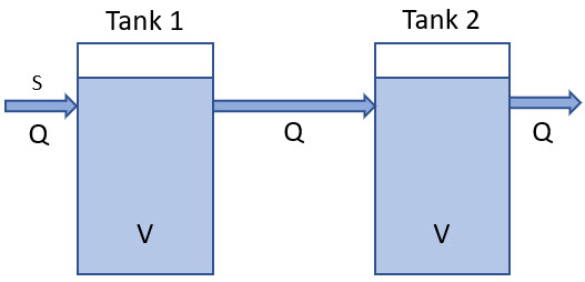
The tanks are always completely and instantaneously mixed and water flows through the tanks at a constant volumetric rate of Q (such that the volumes remain constant).  Initially, both tanks have no chemical mass in them, but at some point we start to inject mass into the inflow to Tank 1 (such that the inflow has a constant concentration of S). Recalling our discussion about boundaries in the previous Lesson, the system includes only the two tanks (and the pipe connecting them). There is a boundary upstream of Tank 1 (the mass flowing in is an external forcing function) and there is a boundary downstream of Tank 2 (we no longer track the mass after it leaves Tank 2).

Given this information, we can write the mass balance equations (one for each compartment, in this case, each tank) in the form of differential equations to represent this system.  We will write these equations in terms of the mass of chemical, M, and the concentration, C, in each of the two tanks:

We can use the volume to convert concentrations to mass, and rewrite these equations in terms of only the mass:

Thinking back to your calculus class, you may recognize these as a system of coupled first-order linear ordinary differential equations. We will discuss how these (and the other equations introduced below) are solved later in this Unit.

The QC (or QM/V) terms represent advection. Advection is the transport of material (e.g., contaminants) via the bulk movement of the medium (typically water) in which those materials are dissolved or suspended. Advection will typically be the dominant transport processes in systems that you will model.

In the simple example described above, we had two equations, one for each “location”, in this case two tanks, each of which were assumed to be well-mixed.  However, what if we had a physical situation in which we could not assume such a well-mixed system?  For example, imagine a tube of cross-sectional area A and length L in which water enters at one end and exits at the other end:

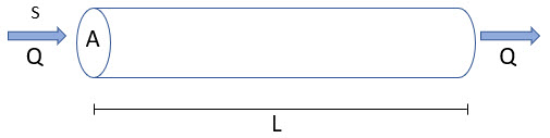
In this case, if we introduced mass into the tube at the upstream end at a constant concentration S (uniformly across the entire cross-sectional area), the concentration would subsequently vary along the tube from 0 to L.  Let’s assume that we can treat the system as fully one-dimensional (i.e., the flow rate and the concentration is constant across a cross-sectional plane normal to the tube). In this case, it can be shown that we could write the governing equation describing that concentration as follows:

where v is the velocity of the flowing water (equal in this simple example to Q/A, where Q is the flow rate and A is the cross-sectional area), and x is the distance along the tube (from 0 to L).

(If you are interested, a nice explanation of the derivation of this - as well as the other equations we will discuss below - is provided in Applied Contaminant Transport Modeling by Zheng and Bennett.)

In this equation, C represents the concentration at any point along the tube (defined by x). Note that this is a partial differential equation, in that C is a function of both time and distance along the tube. (To fully describe this system, we would also need to specify boundary conditions at the upstream and downstream ends of the tube, but for the purposes of the present discussion, we don’t need to worry about this.)

The key point to note is that this is a very different type of equation than when we could simply assume two well-mixed separate tanks.  In particular, in this case, the concentration varies continuously over the tube (i.e., as x varies from 0 to L), and the governing equation (the advective flux) is defined in terms of a concentration gradient (and if we did not impose the assumptions that allowed us to treat the system in only one dimension, we would need to consider concentration gradients in all three dimensions).

Another way to think about this is that whereas when representing parts of your system as well-mixed compartments there is an implicit spatial component to the system (since the compartments are in fact spatially separate), in other cases there is an explicit spatial component to the system that directly impacts mass transport rates. This requires a different approach to solving the equation than did the tank example (as we will discuss starting in Lesson 8).

One final comment about this equation: in the real world this equation would be unlikely to accurately describe the actual concentration variation in time and distance along the tube. If this truly was the correct description of the system, assuming the tube started with no contaminant present, and we started adding contaminant at a constant rate at the upstream end, if we monitored the end of the tube, we would see that the concentration leaving the tube would go from 0 to S (where S is the concentration added at the upstream end) in a sharp vertical step (as shown in the red curve below). This plot of concentration versus time at the end of the tube is referred to as a breakthrough curve.

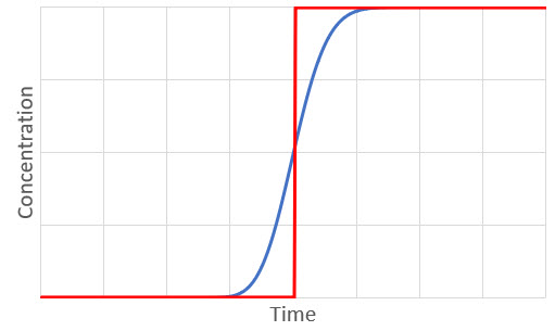
In the real world, however, we would see that this breakthrough would be spread out or dispersed to some extent (as shown in the blue curve). That is, realistically, we can’t explain the behavior using advection alone and need to also represent whatever process is causing this dispersion.

This dispersion occurs because not all of the molecules of the chemical move longitudinally along the tube at the same rate. We will discuss this important process in the next Lesson.