Unit 15 - Modeling Scenarios

Lesson 9 - Exercise: Using Scenarios

Now that we have discussed the various aspects of scenario modeling, in this Lesson we will carry out an Exercise based on what we have learned.

We are going to start with an Example we looked at in Unit 8, Lesson 8. Go to the “Examples” subfolder of the “Basic GoldSim Course” folder you should have downloaded and unzipped to your Desktop, and open a model file named Example4_Deadband_Controller.gsm.

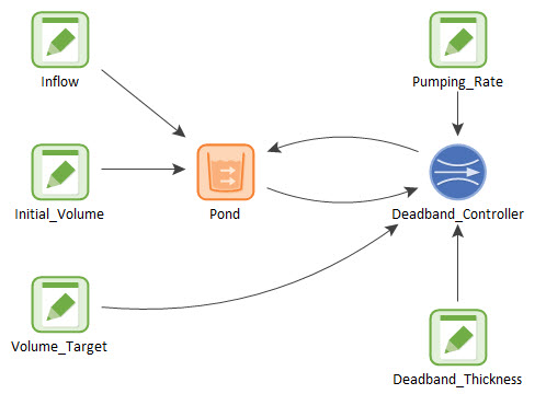
Recall that this model simulated a pond that received a Stochastic inflow. The goal was to maintain the water volume around a particular “target” level. We did this by representing a deadband using a Controller element. The model looks like this:

We are going to make one change to this model to make it a bit more interesting. Let's replace the Inflow Data element with a Stochastic. Define it as an Exponential distribution with a mean of 100 m3/day, and resample the Stochastic every hour (Use On Changed Hour for the trigger). Next, create three scenarios. The only difference between the three scenarios is that the Pumping_Rate will differ: it should take on three different values: 50 m3/day, 100 m3/day and 400 m3/day.

Run the three scenarios and compare the results.

Stop now and try to build and run the model for all three scenarios.

Once you are done with your model, save it to the “MyModels” subfolder of the “Basic GoldSim Course” folder on your desktop (call it Exercise23.gsm). If, and only if, you get stuck, open and look at the worked out Exercise (Exercise23_Dead_Band_Scenarios.gsm in the “Exercises” subfolder) to help you finish the model.

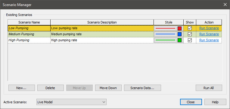
This model should have three scenarios defined, so the Scenario Manager should look something like this:

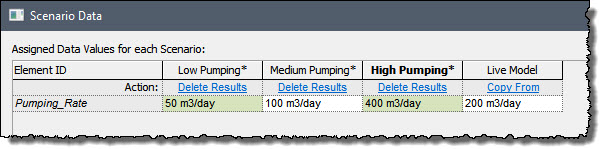
The Scenario Data dialog should look like this:

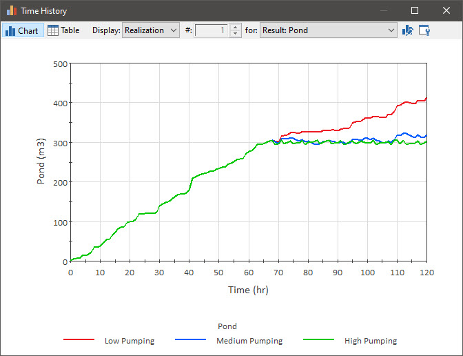
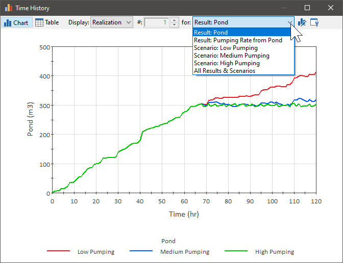
After running the three scenarios, the Time History Result element should look like this:

Note: Your result will not look identical to this, since (as discussed in Unit 13, Lesson 7) your Stochastic element will have a different random number seed.

Note: The y-axis of this model was set to be red in the original model. This, however, is no longer appropriate now that we have scenarios. Press the Chart Style button (second from the right), go to the Y-Axis tab, and in the Style section, set the axis color to black. You can also do the same thing for the Y2-Axis tab.

What you will note here is that the high pumping rate scenario successfully keeps the volume at the target. The medium pumping rate does fairly well (but allows the volume to drift a bit – the rate is not always high enough to keep up with the inflow). The low pumping rate fails - it is too low to keep up with the inflow.

This particular Time History Result is interesting because it actually contains not one, but two different outputs. You can see this by pressing the Edit Properties… button on the far right side of the tool bar:

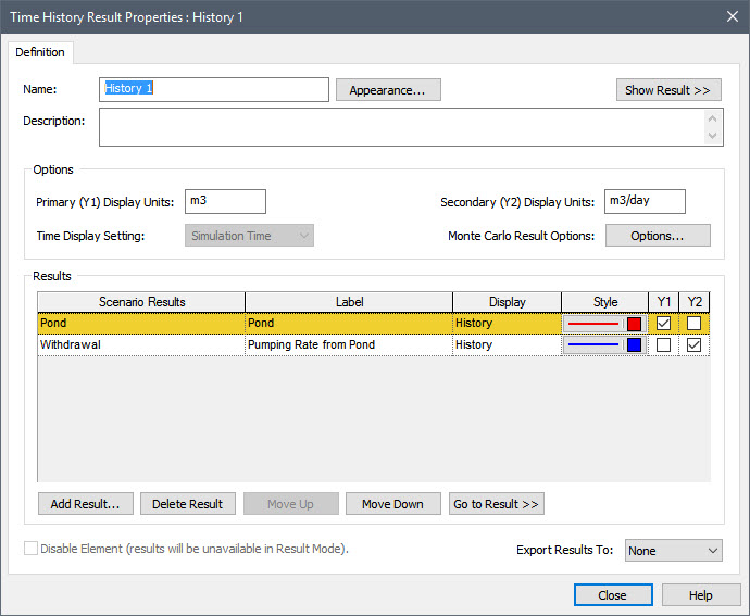
Close the Properties dialog and return to the chart. When we looked at scenarios in Time History Result elements previously, the Time History Result only had a single output. Now we have two. So how does GoldSim handle this? You will note at the top of the chart that there is a for drop-list:

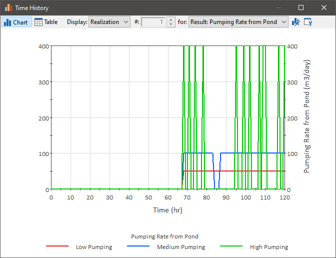
When you have run scenarios and have multiple outputs, you can select what you want to display. If you select one of the first two (with the prefix “Result”), GoldSim displays the three scenarios for that particular output (result). For example, select “Pumping Rate from Pond” and GoldSim will display the pumping rate (rather than the pond volume) for all three scenarios:

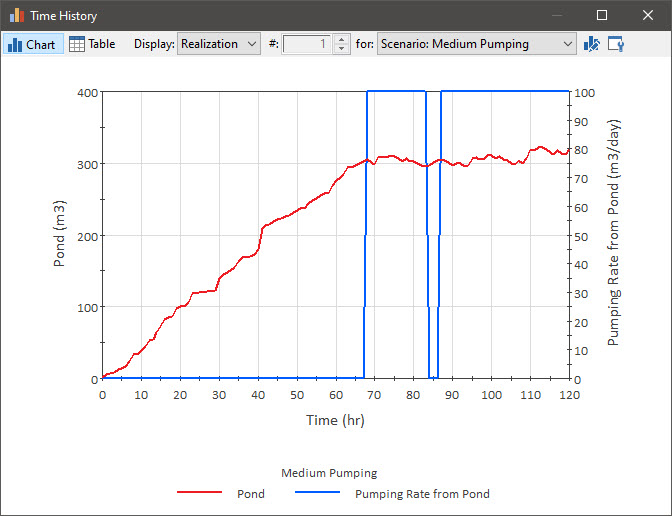
On the other hand, if you select one of the three with the prefix “Scenario”, GoldSim displays the two outputs for that particular scenario:

This feature allows you to effectively display all the scenario results in multiple ways.