Courses: Introduction to GoldSim:
Unit 7 - Modeling Material Flows
Lesson 5 - Understanding the Withdrawal Rate Output of a Reservoir
You will recall that in a previous Lesson (Unit 7, Lesson 2), we noted that a Reservoir always has at least two outputs (a primary output, and at least one secondary output).
We also noted that when you left-click on the output port for an element, it shows all of the element’s outputs (indented under the element name). For example, for a Reservoir with a specified Upper Bound, there are four outputs:
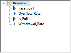
The output with the same name as the element is the primary output, and represents the value of the Reservoir (i.e., the current value of the integral). The Overflow_Rate is the rate at which the Reservoir is overflowing (and is zero if the primary output is below the Upper Bound). The Is_Full output is True if the Reservoir is at its Upper Bound and False otherwise.
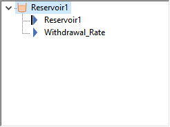
If there is no specified Upper Bound, there are only two outputs:
In both cases, we see that there is always an output named “Withdrawal_Rate”. What does this represent? Recall that Reservoirs have an input named Rate of Change under the “Withdrawal Requests” section (open a Reservoir dialog to see this). Is the “Withdrawal_Rate” output the same thing as this Rate of Change input? The answer is no. These are not the same thing. The Withdrawal Request Rate of Change input is what you want to withdraw from the Reservoir (it is a demand or a request). The “Withdrawal_Rate” output is what is actually withdrawn from the Reservoir (which may be less than the request). In particular, if the Reservoir is above its Lower Bound, the “Withdrawal_Rate” output is identical to the Withdrawal Request Rate of Change input. However, if the Reservoir is at its Lower Bound, the “Withdrawal_Rate” output may be less than the Withdrawal Request Rate of Change input.
The best way to understand this is to look at a very simple example. Start with a new model and insert a Reservoir. Set its Display Units to m3, give it an Initial Value of 258 m3, a Rate of Change in the “Additions” section of 50 m3/day, and a Rate of Change in the “Withdrawal Requests” section of 55 m3/day:
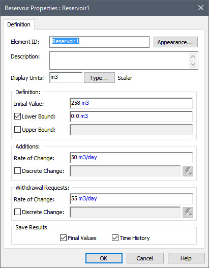
Note: As noted previously, you should never enter values like this directly into a dialog. Instead, you should create Data elements for these inputs (258 m3, 50 m3/day and 55 m3/day) and link the Data element to the input fields. We are entering the inputs directly here simply to quickly illustrate how a Withdrawal_Rate output works.
Now run the model (we will use the default Duration of 100 days and the default timestep of 1 day). When you do so, you will get a warning message. We will revisit this in a moment. For now, ignore it (press No in the warning dialog).
Now plot the Reservoir volume (the primary output) and the Withdrawal_Rate output on the same chart (you should know how to do this now based on the previous Lessons). It will look like this:
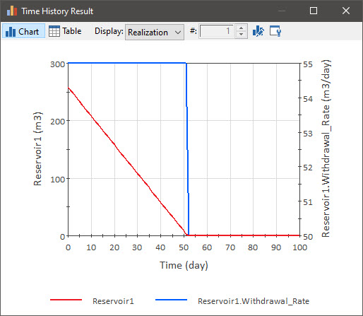
What is happening here? The Withdrawal Request Rate of Change is 5 m3/day greater than the Addition Rate of Change, so we are effectively removing a net of 5 m3/day from the Reservoir. Hence, after approximately 51 days, the Reservoir reaches its Lower Bound (of 0 m3). The Withdrawal_Rate output (plotted on the right-hand axis in the chart above) starts at 55 m3/day. But once the Reservoir is empty, it is reduced to 50 m3/day.
Several things should be noted here:
- While the Reservoir is above its Lower Bound, the Withdrawal_Rate output is identical to the Withdrawal Request Rate of Change (55 m3/day).
- Once the Reservoir reaches its Lower Bound, it is not possible to withdrawal 55 m3/day anymore (as this would cause the Reservoir to go below its specified Lower Bound of 0 m3). However, this does not mean that the Withdrawal_Rate is zero. You can still withdraw some material as long as there is material coming in. In particular, you can withdrawal whatever is flowing in. You just can’t withdraw everything you requested. In this case, the Addition Rate of Change is 50 m3/day. The Withdrawal Request Rate of Change is 55 m3/day (which is more than can be provided). GoldSim responds by saying that the actual Withdrawal_Rate must drop to 50 m3/day. That is, the Reservoir remains empty, and everything that is added is immediately withdrawn.
The implication of this is that if you are withdrawing material from one Reservoir and directing it to some other location (e.g., another Reservoir), and the first Reservoir can potentially reach its Lower Bound, it is critical that you reference the Withdrawal_Rate output when specifying the rate at which material is added to the other location to ensure that you are actually conserving the material.
To illustrate this, consider an example in which water is pumped from Pond1 to Pond2. One way to build this model is as follows:
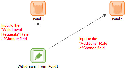
In this case, the Data element serves as both an input to Pond1 (as the Withdrawal Request Rate of Change) and as an input to Pond2 (as the Addition Rate of Change). However, this would be incorrect and could cause you to artificially create water in this model! If Pond1 hits its Lower Bound, the Data element no longer represents the actual Addition Rate of Change to Pond2. The actual Addition Rate of Change might be less than Withdrawal_from_Pond1. That is, the Data element represents the requested withdrawal rate, but is not necessarily the actual withdrawal rate.
The correct structure for this model would look like this:
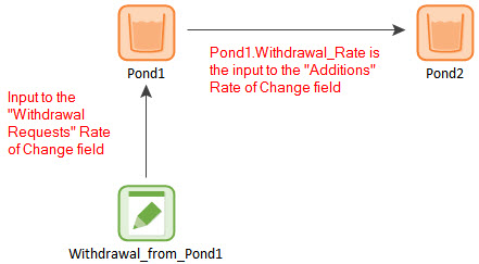
In this case, the Addition Rate of Change input for Pond2 is Pond1.Withdrawal_Rate. This ensures that the actual (as opposed to the requested) withdrawal rate from Pond1 is added to Pond2.
It should also be noted that such a structure makes the model logic clearer (i.e., Pond1 flows to Pond2).
Because ignoring the Withdrawal_Rate output when a Reservoir reaches its Lower Bound (and the withdrawal is restricted) could result in a significant error in your model, GoldSim generates a warning message whenever a Reservoir reaches its Lower Bound such that the requested withdrawal cannot be delivered AND the Withdrawal_Rate output is not referenced by another element.
Recall that when you ran the simple model we built above, a message appeared. The message noted that there was a warning, and asked if you wish to view the Run Log. As noted previously, if a simulation generates any warning messages during the run (as was the case here) you will immediately be prompted to view the Run Log when the simulation completes. The Run Log can also be viewed at any time after a simulation is completed by selecting Run|View Run Log in the main menu. Let’s do that now.
Note the “Warning and Errors” section at the bottom:

The warning says that the outflow is restricted, but the Withdrawal_Rate is not being referenced elsewhere in the model. This is not necessarily a problem (hence it is not a fatal error), as you may not be interested in tracking the withdrawal. But GoldSim provides the warning just in case you are interested in tracking the withdrawal, but simply forgot to track it (or are tracking it incorrectly).
Finally, before we finish this Lesson, let’s look at the result of the simple model we built above one more time. You will note that the Reservoir appears to empty at 52 days. But is that really when it emptied? Actually, that is not when it reached zero. Knowing the initial volume and the addition and withdrawal rate, you can easily compute by hand when the volume would reach zero. And it turns out that it actually reaches zero at 51.6 days. This is between GoldSim timesteps (recall we specified a 1 day timestep).
So how does GoldSim handle this? In fact, the Run Log that we viewed above told us exactly how GoldSim handled this. The Run Log indicates that the Reservoir reached the Lower Bound at 51.6 days.
As we discussed in the previous Lesson, in some cases, certain events may occur between scheduled updates of a model, and waiting for the next scheduled update could decrease the accuracy of the simulation. Such events trigger what is referred to as an “unscheduled update” of the model. There are a number of events that can trigger an unscheduled update to occur. We’ve already discussed that reaching the Upper Bound of a Reservoir triggers an unscheduled update. Reaching a Lower Bound of a Reservoir also triggers an unscheduled update, and that is what has happened here.
As we noted previously, for the most part, you don’t need to be aware of these updates; GoldSim carries them out “silently” in order to more accurately simulate the system. Keep in mind, however, that because of the fact that these timesteps are inserted it is important to understand that the value of an output (in this case, the Withdrawal_Rate) reported at a particular time represents the instantaneous value at that point in time, and does not represent the average value over the timestep.
This point is apparent from looking at a table view of the result of the simple model:
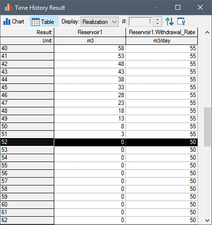
The withdrawal rate at 52 days (50 m3/day) does not represent the average overflow rate over the previous day (since we know that it actually did not become constrained and reduced from 55 m3/day until 51.6 days). It represents the instantaneous value at exactly 52 days.
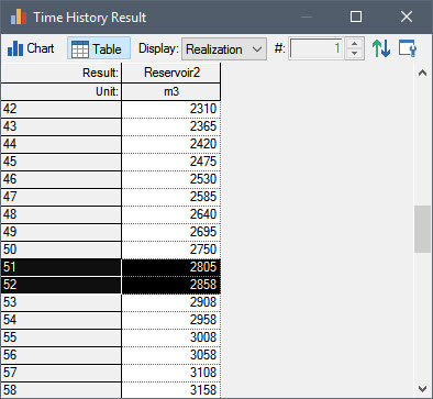
It is important to understand, however, that even though GoldSim only reports instantaneous values at each scheduled timestep, GoldSim correctly captures the fact that the withdrawal rate did not become constrained until 51.6 days (because GoldSim “silently” inserted a timestep at that time). One way to see this would be to route the actual withdrawal (the Withdrawal_Rate output) into the Addition Rate of Change of another Reservoir and see how the volume of that second Reservoir changed between 51 and 52 days. If you do so, you will note that the volume change between 51 days and 52 days is equal to (55 m3/day * 0.6 days) + (50 m3/day * 0.4 days) = 53 m3:
Note: Recall from the previous Lesson you can actually see the impact of an unscheduled update that was inserted by including unscheduled updates in time history results.