Lesson 3 - Exercise: Modeling an Overflowing Pond

We are now ready to do our next Exercise. We are going to create a new model (this Exercise will not build on a previous one).

In this Exercise, we are going to simulate a pond that fills with water.  In particular, we will assume the following:

• The initial volume of the pond is 1200 m3
• The capacity (upper bound) of the pond is 35000 m3
• There is a constant inflow to the pond of 1000 m3/day

We will run the model for 50 days and use a 1 day timestep.

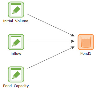
So to create this very simple model, you will need to create three Data elements (for the initial volume, capacity and inflow), and a Reservoir element to represent the pond.

We want to plot the pond volume and overflow rate on the same chart (using a Result element).  But you don’t need to do that now.  We will walk through that step together below.

Stop now and try to build and run the model.

Once you are done with your model, save it to the “MyModels” subfolder of the “Basic GoldSim Course” folder on your desktop (call it Exercise4.gsm), as we will build upon this in a later Lesson. If, and only if, you get stuck, open and look at the worked out Exercise (Exercise4_Overflow.gsm in the “Exercises” subfolder) to help you finish the model.

One you have built the model, run it. Note that when you run the model you will see a warning message:

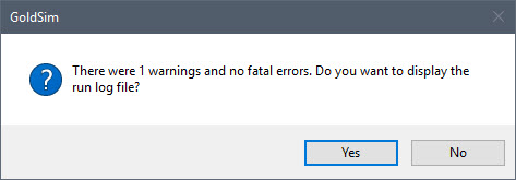
For now, you can ignore this (just press No).  We will discuss this message below.

First let’s look at the model.

If you were lazy, you could actually have defined the Reservoir such that it looked like this:

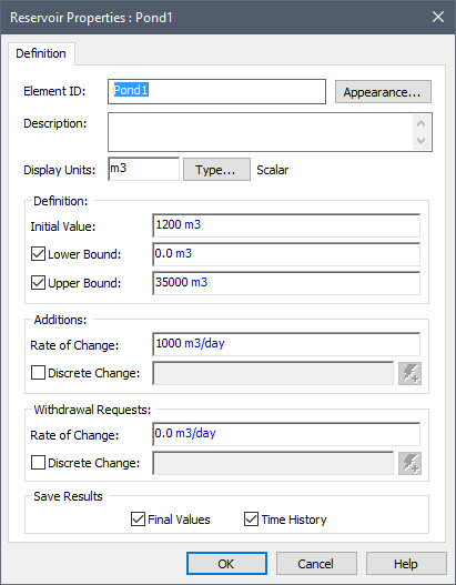
As we mentioned when discussing the Selector in a previous Lesson (Unit 6, Lesson 11), while defining an element this way is not technically incorrect (it will produce the correct answer), it is stylistically incorrect. Why?  Because it buries input variables (1200 m3, 1000 m3/day, 35000 m3) directly inside the element.  All inputs in a model should always be entered using input elements (e.g., Data elements).  This makes the model more transparent, and less likely to contain errors.  For example, assume that the inflow rate (1000 m3/day) needed to be used in two different places in the model.  By defining this inflow as a Data element, you could simply reference the same Data element in both places.  If you needed to change the value, you would only need to change it in one place.

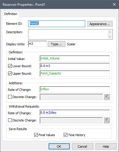
So instead, your pond should look like this:

And the model should look like this:

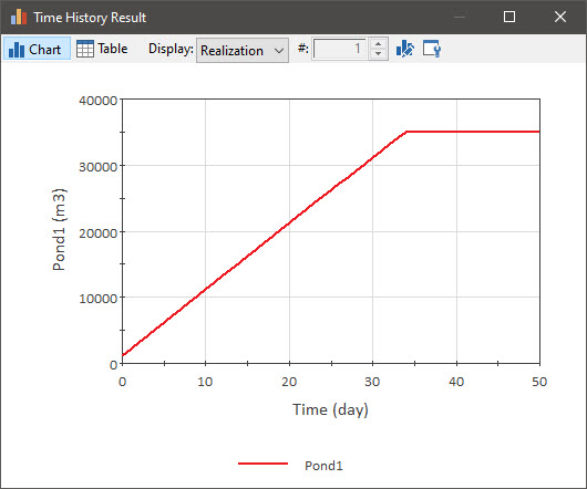
Now let’s run the model and look at the results. Right-clicking on the Reservoir element (to display the context menu) and selecting (left-clicking) Time History Result… will display a time history chart of the pond volume:

The button furthest to the right at the top of the chart window is the Edit Properties button:

Press that button to view the Result Properties dialog:

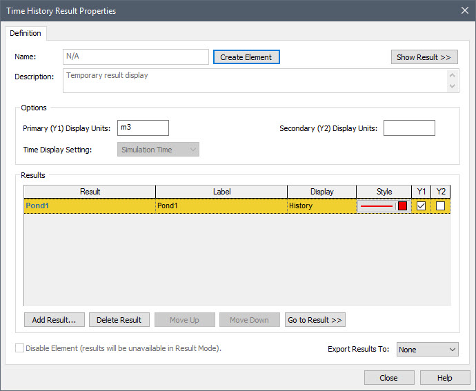
Before we go any further, let’s turn this into a Result element by pressing Create Element. After doing so, you will be able to edit the name of the element.  Name it “History Plot”.

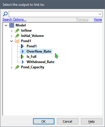
Now press the Add Result… button to add another output to the chart. Expand the Reservoir and select the Overflow_Rate:

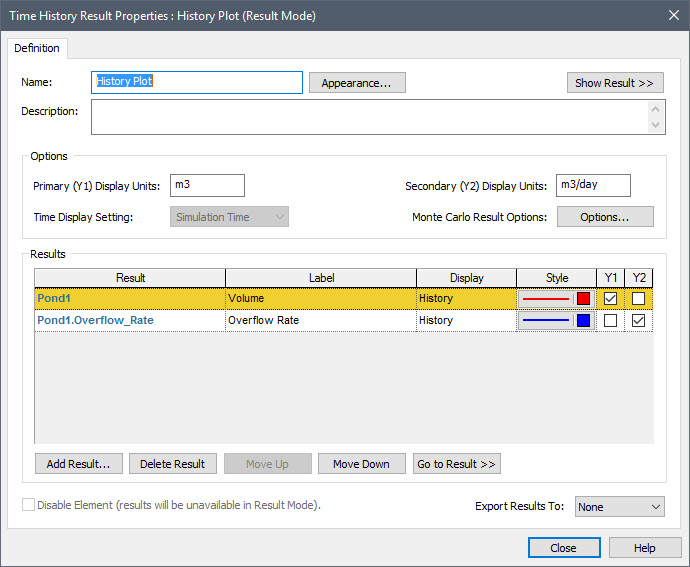
The Result Properties dialog will now look like this:

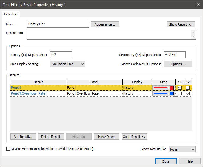
Note that the overflow rate is assigned to the Y2-axis. Let’s make the following changes in this dialog:

• Change the Label for the two outputs: Let’s change the Label for the first item (the volume) to “Volume” and the Label for the second item (the overflow rate) to “Overflow Rate”.

The dialog should now look like this:

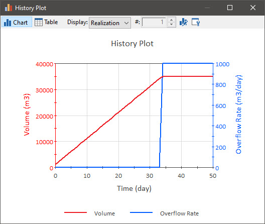
Press Show Result>>.  The chart should look like this:

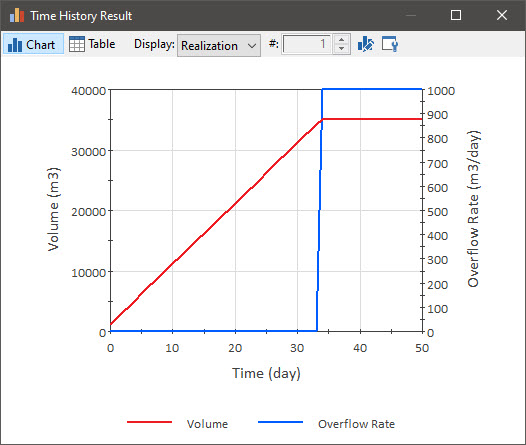
Note that as soon as the volume reached the Upper Bound, the pond started to overflow (i.e., the Overflow Rate went from zero to 1000 m3/day).

This is a good opportunity to explore some of the formatting options available for charts. 

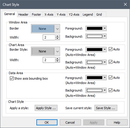
Press the Chart style button:

When you do so, a Chart Style dialog will appear (next to the chart):

For the most part, this dialog is self-explanatory, but there are a few points worth discussing here. Let’s start by going to the Y-Axis tab.  It will look like this:

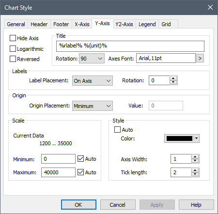
This tab allows you to change the format of the Y-axis.  Most of the options here are straightforward.  Note, however, the Title:

%rlabel% %(unit)%

What does this mean?  Anything that starts and ends with “%” is known as a keyword. Keywords are dynamically replaced with the appropriate text.  There are a wide variety of keywords available within GoldSim. You can access a full list by right-clicking in any Title or Text input field in the chart style dialog (such fields are available on the Header, Footer and Axis tabs). 

In this case, the keyword %rlabel% inserts the label for the first output assigned to that axis (as defined in the Result Properties dialog).  The keyword %(unit)% inserts the actual units (in parentheses) being displayed.  The axis Title defaults to using these keywords, but if you wished to, you could change the Title to anything you wish.  In this case, we will keep this Title.

Before we leave this tab, let’s make one change. Let’s change the axis Color from black to red.

Now let’s go to the Y2-Axis tab.  In this tab, let’s change the axis Color from black to blue. Press OK to close the dialog.  The chart will now look like this:

It should now be obvious why we made these color changes.  By doing so, it is much clearer which axis corresponds to which output.  This is a nice little trick that you can use when plotting results that use multiple Y-axes.

Once you are happy with this file, remember to save it to the “MyModels” subfolder of the “Basic GoldSim Course” folder on your desktop (call it Exercise4.gsm). We will explore the results of this model further in the next Lesson.

However, before moving on, we need to discuss one additional issue.  Recall that when you ran the model, a warning was posted. We ignored this warning, but as a general rule, you should never do so.  Let’s take a closer look at that warning now:

The message notes that there was a warning, and asks if you wish to view the Run Log. Whenever you run a GoldSim model, a Run Log is produced. The Run Log contains basic information regarding the simulation (e.g., the version of the program, the date, the simulation length), and any warning and error messages that were generated.

If a simulation generates any warning messages during the run (as was the case here) you will immediately be prompted to view the Run Log when the simulation completes. The Run Log can also be viewed at any time after a simulation is completed by selecting Run|View Run Log in the main menu. Let’s do that now.

Note the “Warning and Errors” section at the bottom:

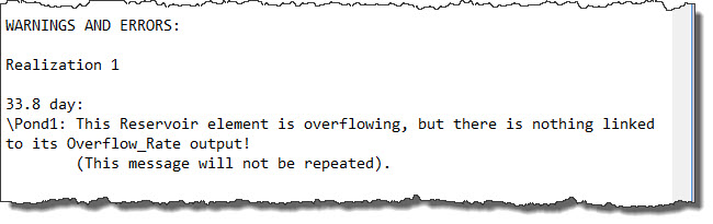
The warning says that a Reservoir is overflowing, but the Overflow_Rate is not being referenced elsewhere in the model.  Hence, that material is “lost” from the system. This is not necessarily a problem (hence it is not a fatal error), as you may no longer be interested in tracking whatever overflows.  But GoldSim provides the warning just in case you are interested in tracking the overflow (e.g., by routing it somewhere), but simply forgot to do so.  In a subsequent Lesson, we will explore how you might go about routing such an overflow.