Courses: Introduction to GoldSim:
Unit 10 - Building Hierarchical Models
Lesson 5 - Tools for Exploring Complex Hierarchical Models
Now that we have learned the basics of creating and navigating Containers, in this Lesson, we’ll discuss a number of tools that are available for exploring and understanding complex hierarchical models.
The easiest way to do this is to look at a pre-built model. You will find this model the “Examples” subfolder of the “Basic GoldSim Course” folder you should have downloaded and unzipped to your Desktop. In that folder open a model file named Example16_Dependencies.gsm:
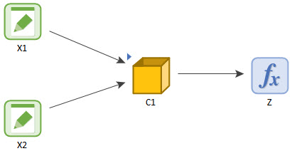
What can we learn from simply looking at the elements in the graphics pane? For example, can we conclude that Z is a function of X2? You might be tempted to answer “Yes”, but this would be incorrect. All we can conclude from viewing these elements at this point is that at least one element within the Container C1 is a function of X2, and Z is a function of at least one element within C1. That, of course, does not imply that Z is a function of X2.
In fact, if you explore this model (by looking inside C1), you will see that Z is, in fact, not a function of X2. There is an element inside C1 (Y3) that is a function of X2, but Z is not a function of Y3. Hence, Z is not a function of X2.
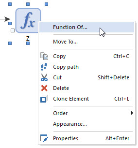
But is there an easier way to determine this? In this simple model, it was easy to answer the question by quickly exploring the model. But in a complex model (with many layers of Containers), this would be very difficult. Fortunately, GoldSim provides a very powerful tool for answering this question. Return to the top level of the model and right-click on Z. In the context menu, you will see an option labeled Function Of… :
If you click this, a specialized browser window is displayed:
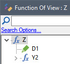
It starts with the selected element, and only shows those elements which directly affect that element (i.e., those elements which the selected element is a function of). In the above example, it indicates that Z is a direct function of D1 and Y2. Note, however, that the tree can be expanded for Y2. Do that now (by clicking the plus sign next to Y2). Continue to expand the tree until it can no longer be expanded. It will look like this:
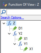
This indicates that Y2 is a function of X1 and Y1, and that Y1 is also a function of X1 (i.e., an item can show up multiple times in such a tree). This shows the entire dependency structure for Z (and clearly indicates that it is not a function of X2, as X2 does not appear in the tree).
Of course, in a complex model, this tree could be very complex (having tens or hundreds of branches) so simply opening it in this way would not be feasible. Instead, you would use the search bar. If you enter the name of the element of interest (in this case X2, as we want to know if Z is a function of X2) and press the search button (the magnifying glass), GoldSim will search the entire tree (all branches). In this example, it would not find a match.
We could have learned the same information by right-clicking on X2. In that context menu, you will see an option labeled Affects… If you click this, a similar browser window is displayed:
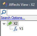
This view of the model starts with the selected element, and only shows those elements which are a function of that element (i.e., those elements which the selected element affects).
In this case, it is clear that X2 affects Y3, and nothing else.
Note: If you right-click on an element that is not a function of any other elements, Function Of… is not displayed in the context menu. Likewise, If you right-click on an element that does not affect any other elements, Affects… is not displayed in the context menu.
It should be easy to see how the Function Of and Affects browsers provide a powerful way to explore a complex model.
Let’s look again at the model and ask the question: “Which element(s) does X1 directly affect inside of C1?”. We just saw that we could use the Affects view to see this. But we can also see this information in an even simpler way. Hold your cursor over the influence connecting X1 to C1 and the following tool-tip will be displayed:
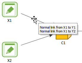
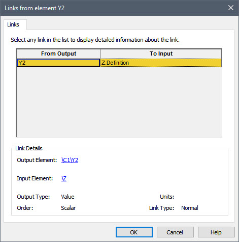
The tool-tip indicates that X1 is linked to Y1 and Y2. If we double-click on the influence, we can see even more information regarding these links:
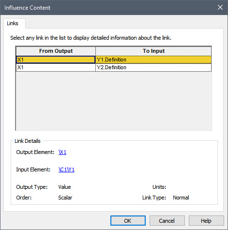
Each link is represented by a row: an Output (where it originates), and an Input (where it ends). When you select a specific link in the top part of the dialog, it is highlighted in yellow and its details are displayed in the bottom part of the dialog. The details include a listing of the full path of the input or output. The "path" refers to the containment path (e.g., A\B\C\X would indicate that the element named "X" is located in Container C, which is inside Container B, which is inside Container A). You can jump to the element associated with a particular input or output by clicking on the path in the Link Details section. The details also describe the Output Type (e.g., value, condition), Units, and Order (e.g., Scalar, Vector or Matrix).
Let’s explore one other critical tool for understanding hierarchical models by entering the C1 container. It looks like this:
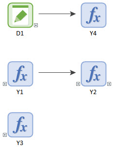
The first thing you will notice is that some of the elements have only an input port (small box on the left-side of the element), some elements only have an output port (small box on the right-side of the element), some have both, and some have none at all! What is going on here?
We’ve mentioned input and output ports briefly in previous Units. Let’s revisit them again now. All elements have ports, but by default, ports are only shown if they have some useful information to display.
Note: The behavior described above for ports (they are only shown if they have information to display) is the default behavior. However, via the Model | Options dialog you have the option to always show them or always hide them. It is recommended, however, that you do not change this default behavior.
There are two primary types of information that ports display:
- As has been mentioned in previous Units, output ports are shown in Result Mode (if the element has results to display).
- Input and output ports are also displayed in order to indicate that the element is linked to an element in another Container (if the element is linked to an element in the same Container, this is indicated by showing an influence arrow). In this case, the port is displayed with a dot in the middle of it.
This second item provides an important tool and visual cue when you are viewing a model. In the example above, by simply looking at the graphics pane, we can immediately draw the following conclusions:
- Y1, Y2 and Y3 are functions of (have inputs from) one or more elements outside of this Container.
- D1 and Y2 affect (have outputs to) one or more elements outside of this Container.
- Y3 and Y4 are “dead-ends”; they have no effect on any elements inside the Container (as there are no influences leaving them), and they have no effect on any elements outside of the Container.
If you right-click on one of these input or output ports, you can choose to show the links to or from the element:
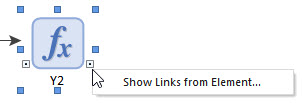
This will display dialog similar to the one displayed when double-clicking on an influence:
There is one additional tool for exploring complex models that should be noted, and that is the ability to search the model through the browser. In particular, you can find any element in the model by using the Find button in the main GoldSim toolbar:

If you press this button, the following dialog will appear:
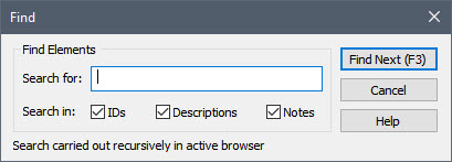
Enter a string and GoldSim will search recursively through the browser. You can choose to search element IDs, Description and Notes (discussed in Unit 16) for the string.