Courses: Introduction to GoldSim:
Unit 10 - Building Hierarchical Models
Lesson 4 - Exercise: Organizing a Model Using Containers
Now that we have learned the basics of creating and navigating Containers, in this Lesson, we’ll do a simple Exercise to give you some more practice with Containers.
We are going to start with a model we built in a previous Exercise. In particular, we are going to revisit the model of the leaky pipeline that we built in the previous Unit (Unit 9, Lesson 4). You should have saved that model and named it Exercise9.gsm. Open the model now. (If you failed to save that model, you can find the Exercise, named Exercise9_Leaky_Pipeline.gsm, in the “Exercises” subfolder of the “Basic GoldSim Course” folder you should have downloaded and unzipped to your Desktop.)
The model should look something like this:
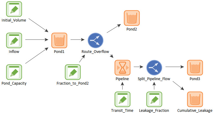
(The model should also contain at least one Result element, not shown here).
For this Exercise, use Containers to reorganize the model. Note that there is no single “correct” way to do this. Simply use the skills you learned in the previous Lesson to create some Containers and think about ways that this model could be reorganized.
Stop now and try to edit the model. There is no reason to run it.
Once you are done with your model, save it to the “MyModels” subfolder of the “Basic GoldSim Course” folder on your desktop (call it Exercise12.gsm). If, and only if, you get stuck, open and look at the worked out Exercise (Exercise12_Pipeline_Containers.gsm in the “Exercises” subfolder) to help you finish the model.
As mentioned above, there is no single “correct” way to organize this model. There are multiple ways to approach this. A common approach, however, might result in a structure that looks like this at the top level:
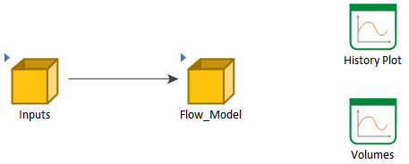
We have simply separated the model into two different Containers. All of the Data elements are in the Inputs Container:

The other elements (the actual computational elements) are in the Flow_Model Container:
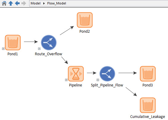
The two Result elements are simply left in the top level of the model for easy access.
It is obvious how this makes the model easier to view and understand.
Of course, we could have further sub-divided the Flow_Model Container into additional Containers, but in this case, it would not add any clarity to do so (and in fact, would likely make the model harder rather than easier, to follow).
Before we leave this Exercise, let’s do one additional thing. While this model is still open, open a second instance of GoldSim (so there should be two instances of GoldSim in your Windows Task Bar). Select one of the Containers you created in the model (e.g., in the example above, the Container named “Flow_Model”). Press Ctrl-C to copy it to the clipboard. Now go to the other instance of GoldSim (an empty model). Place your cursor in the graphics pane and press Ctrl-P to paste the Container from the other model into this new model. When you do so, GoldSim will display an error dialog that looks something like this:
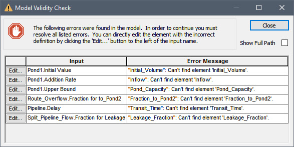
This dialog is simply reporting that it cannot find some of the outputs referenced by the pasted Container. This, of course, is to be expected, as only a portion of the entire model was pasted into the new model. Obviously, when you paste such a Container into another model, you would need to ensure (e.g., by subsequently creating or renaming elements) that any required inputs that were not pasted with the Container (and are likely to be different from those in the original model) are present in the new model. What this simple task illustrates, however, is the reusability of Containers. The ability to copy and paste a Container from one model to another facilitates the creation of a library of documented and verified sub-systems. Such a library could be used within an organization to quickly and efficiently build complex models.