Courses: Introduction to GoldSim:
Unit 12 - Probabilistic Simulation: Part I
Lesson 10 - Creating Correlations and Displaying Multi-Variate Results
In this Lesson, we will discuss in detail how you can create (and display) correlations between parameters in GoldSim. To do so, we will examine another Example model. Go to the “Examples” subfolder of the “Basic GoldSim Course” folder you should have downloaded and unzipped to your Desktop, and open a model file named Example21_Correlation.gsm.
This is a model of an evaporating pond that is similar to a model we examined in Lesson 7. The model looks like this:
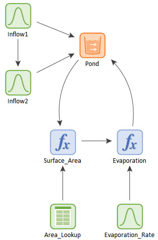
You should notice the following:
- We have defined the Evaporation_Rate as a Stochastic element.
- There are two inflows to the Pond, and both are represented by Stochastic elements.
Hence, this model has three uncertain inputs. Now double-click on Inflow2:
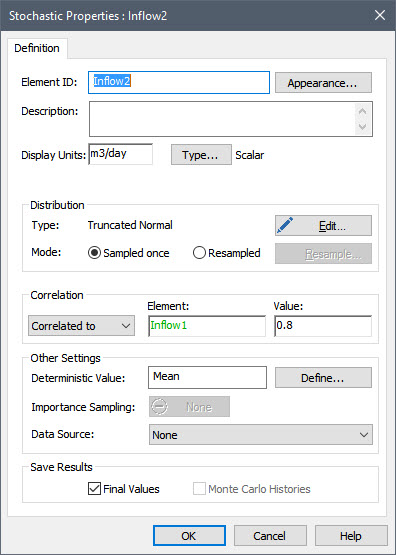
Note that the bottom portion of the Stochastic dialog is expanded. This is because we have used this portion of the dialog (accessed via a More button) to specify that Inflow2 is correlated to Inflow1. In particular, we have specified a correlation coefficient of 0.8. This indicates that the two inflows are strongly positively correlated (if one is high, the other is also likely to be high). This makes physical sense, as the two inflows can be imagined to both be dependent on rainfall.
So what does it mean if these are correlated? Let’s run the model now to find out (the model is set to run for 1000 realizations). To explore the results in this model, we are going to introduce a third type of result display that we have not yet seen: a multi-variate result. Multi-variate results allow you to analyze and compare multiple outputs.
After running the model, right-click on Inflow1 and select Multi-Variate Result… When you do so, the following dialog will appear:
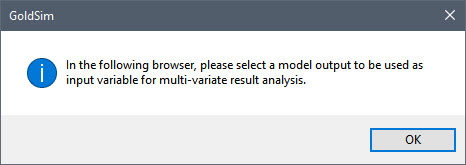
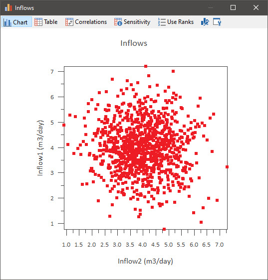
When you press OK, a browser will appear allowing you to select a variable (i.e., another output in the model that we can analyze with respect to Inflow1). From the browser, select Inflow2. After doing so, the following chart will be displayed:
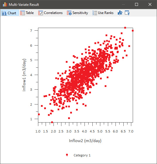
This is a scatter plot of the two variables showing the results for all 1000 realizations. The fact that they are positively correlated is obvious here. Before we close this plot, let’s do two additional things. First, right-click in the chart and clear View|Show Legend. By default, the legend is turned on, and it labels different result “categories”. In this model, we have only a single category. We will discuss how categories can be defined and used in the next Unit.
Like other results, we can create a Multi-Variate Result element. Let’s do so now. At the top of the dialog you will see the Edit Properties button:

Press this now and the following dialog will be displayed (the result display will not be closed, so that both dialogs will remain open):
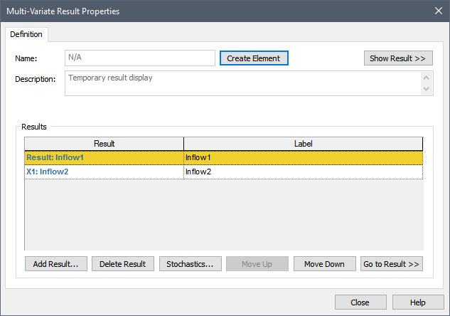
The first row shows the “result” (in this case Inflow1). We are evaluating other outputs with respect to this result. In this example, the other output is Inflow2. We could actually add more outputs here if we wanted to (but we won’t do that now). Instead, let’s press the Create Element button. Name this element “Inflows”.
Close the Result Properties dialog and the display itself, and return to Edit Mode. Now open Inflow2 again, and set the Value for the correlation to 0. Rerun the model, and open the Result element you just created to view the scatter plot again:
Clearly, the two inflows are no longer correlated. As another experiment, set the Value to 1.0. If you do that, you will note that the inflows are perfectly correlated (they form a straight line).
Let’s now examine results for the rest of the model. Before doing so, however, close the display, return to Edit Mode, and reset the Value for the correlation for Inflow2 to 0.8. Don’t rerun the model yet. First, double-click on a different Multi-Variate Result element you will see in the model named “Uncertainty Analysis”:
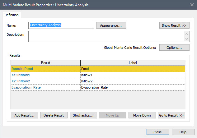
As can be seen, this element is set up so that the Pond is the first output in the list. As we shall see, this has important implications for the analysis that is displayed.
Close the dialog and run the model. Open the “Uncertainty Analysis” Result element:
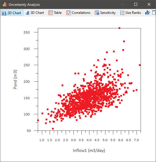
By default, a scatter plot is displayed. The first output in the list (Pond) is displayed on the Y-axis, and the second output in the list (Inflow1) is displayed on the X-axis. As can be seen, as you would expect, the final Pond volume is positively correlated with the inflow.
Note the buttons at the top of this dialog. These represent the various displays available for a Multi-Variate result. If you press the 3D Chart button, a 3D scatter plot will be displayed (using the first 3 outputs in the list). You can rotate the view by using the Up, Down, Left and Right keys.
Of greater value is the Correlations button:
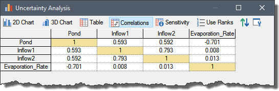
This displays a correlation matrix for the selected outputs. A correlation matrix consists of a table whose column and row headers are identical, and list all of the outputs in the Result Properties dialog. The table entry for a particular row/column pair is the correlation coefficient for that pair of variables. The correlation coefficient takes on a value between –1 and 1, 1 being a perfect positive correlation, -1 being a perfect negative correlation. Because the rows and columns are identical, a correlation matrix is symmetrical on either side of its diagonal.
In this particular example, there are several things worth noting:
- If you examine the first column, you will note that the two inflows have a positive correlation with the resulting Pond volume (the higher the inflow, the higher the volume), and the Evaporation Rate has a negative correlation with the resulting Pond volume (the higher the Evaporation Rate, the lower the volume). This, of course, makes sense physically.
- The third row, second column (or alternatively, the second row, third column) shows the computed correlation between the inputs Inflow1 and Inflow2. It is very close to 0.8 (which is what was specified as the Value for the correlation coefficient). As the number of realizations increases, this computed value would converge to the specified value of 0.8.
Now press the Sensitivity button:
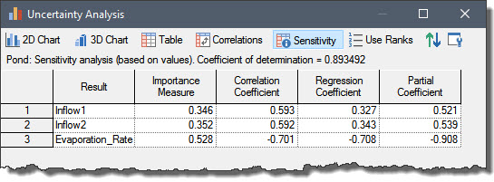
This is one of the most powerful options for analyzing multi-variate results. The table displays the sensitivity of the first output in the list of results in the Result Properties dialog (in this case Pond) to the selected input variables (all the other outputs in the list of results in the Result Properties dialog).
The third column in the table (Correlation Coefficient) displays the same information shown by the Correlation button. The other columns show a variety of other statistical measures. The meaning of each of these is discussed in GoldSim Help.
The analyses provided by the Correlations and Sensitivity buttons are important because one of the key purposes of probabilistic simulation modeling is not just to make predictions, but to identify those parameters that are contributing the most to the uncertainty in results. By doing so, you can determine the most effective way to reduce the uncertainty in your predictions. The analyses provided by these buttons can help to do that.
Note: If you want to carry out more advanced uncertainty and sensitivity analyses, you can do so by exporting all of the results and using a specialized statistical analysis tool.