Courses: Introduction to GoldSim:
Unit 12 - Probabilistic Simulation: Part I
Lesson 8 - Exercise: Using a Stochastic Element
Now that we have learned the basics of probabilistic simulation and explored a few examples, let’s do an Exercise to actually create and use a Stochastic element.
We are going to start with a model we built in a previous Exercise. You should have saved a model named Exercise5.gsm. Open the model now. (If you failed to save that model, you can find the Exercise, named Exercise5_Route_Overflow.gsm, in the “Exercises” subfolder of the “Basic GoldSim Course” folder you should have downloaded and unzipped to your Desktop.)
Open that model and refresh your memory on what we did in that simple model. Recall that this model simulated a pond that received an inflow. The pond has an Upper Bound, and when the volume reaches that level, it overflows into two other ponds (70% to one and 30% to the other).
Note: This model was originally built using Reservoirs for the stocks of material (water) instead of Pools (as we had not yet introduced Pools). If we were to build this model from the beginning again, it would be best practice to use Pools, as they are more powerful and flexible for material management problems (although in this case, that extra power and flexibility is not required). Since the model already exists, however, we will continue to use Reservoirs for the stocks.
We are going to make one simple change to this model: replace the Inflow (which is a Data element with a value of 1000 m3/day) with a Stochastic. Define the Stochastic as an Exponential distribution with a Mean of 500 m3/day. Then change the Simulation Settings so that model is run for 100 realizations.
Stop now and try to build and run the model.
Once you are done with your model, save it to the “MyModels” subfolder of the “Basic GoldSim Course” folder on your desktop (call it Exercise17.gsm). If, and only if, you get stuck, open and look at the worked out Exercise (Exercise17_ Overflow_Uncertain.gsm in the “Exercises” subfolder) to help you finish the model.
Note that the definition for the Inflow should look like this:
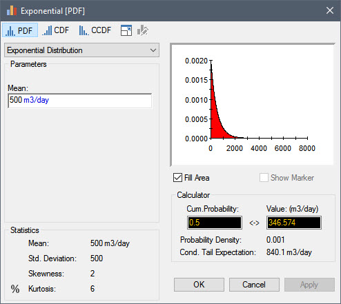
So what we are saying here is that we are uncertain about the Inflow, and that it could range anywhere from a very small value to almost 3000 m3/day.
Double-click on the “Pond Volumes” Time History Result element. This element was set up to be used to display results for all three ponds. By default it is showing the results for the first realization (Display is set to “Realization”):
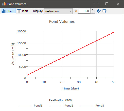
Note: If you built the model yourself (instead of opening the completed model), your first realization will not look identical to this! Why? We will discuss this in detail in the next Unit, but for now if is sufficient to simply note that the random numbers used to sample the distributions were different, and hence the results will not be identical (although statistically the results are consistent and, as we will discuss later, would converge as we increase the number of realizations).
You can toggle through the spin control to view other realizations. You will see in most of the realizations (around 75% of the time) Pond1 never overflows (i.e., a low Inflow value was sampled) and hence Pond2 and Pond3 always have a zero volume. In some of the realizations it does overflow (i.e., a high Inflow value was sampled), and hence Pond2 and Pond3 do receive water (and hence at some point have non-zero values).
Change the Display to “All Realizations”:
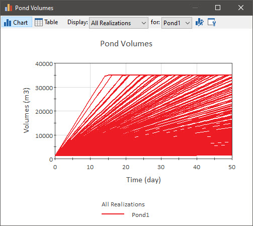
Note that in this case, only one output (in this case, Pond1) is shown. This is because when a display consists of more than a single line (which is the case here for “All Realizations” as well as for “Probabilities”), it is not possible to show more than one output at a time – the display would be a jumbled mess. So in these cases, you can use the drop-list (labeled “for”) just to the right of the Display drop-list to select the output that you want to display. Use that drop-list now to view Pond2 and Pond3.
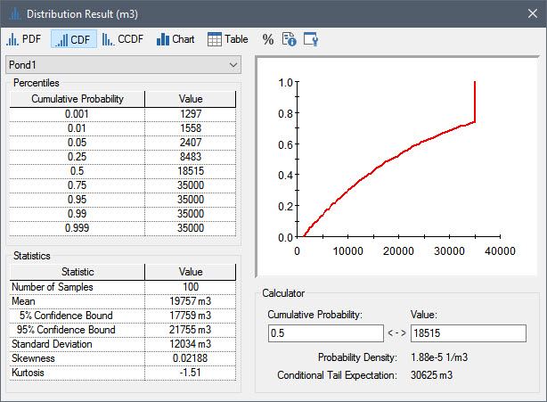
Close the Time History Result element, and right-click on Pond1 and select Distribution Result… to view the distribution of the final value of the volume (i.e., the value at the end of the 50 day simulation):
Note: When viewing tables like this, you can press Alt-Right and Alt-Left to display more or less significant figures.
Note that this is a CDF (the y-axis shows the probability of being less than or equal to the corresponding value on the x-axis).
The upper left-hand portion of the dialog displays a number of selected Percentiles. We could use the Calculator to view the Value for a percentile not listed here by entering the desired percentile into the Cumulative Probability field of the Calculator. For example, here is the 60th percentile:
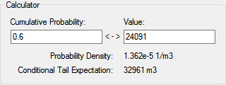
This indicates that the 60th percentile is equal to 24,091 m3.
Note that the CDF becomes vertical at 35000 m3 (the Upper Bound). From the chart, you can see that the point where the line goes vertical is approximately 0.7 to 0.75. This indicates that there is a 70% to 75% chance of the final value being less than 35000 m3 (i.e., of the pond not overflowing in 50 days).
If we wanted to see the actual computed cumulative probability (instead of trying to estimate it from the chart), we could just enter a value just below 35000 (e.g., 34999.99) into the Value field of the Calculator:
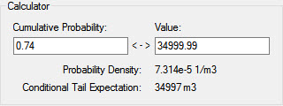
This indicates that there is a 74% chance of the value being less than or equal to 34999.99.
(We entered a value just under 35000 here because the Calculator returns the probability of being less than or equal to the value. Hence, if we would have entered 35000, it would have returned 100%.)
The lower left-hand portion of the dialog displays a number of Statistics for the result distribution.
It is important to note that if you do this calculation (assuming you built your model instead of opening the completed model), your Calculator will return slightly different results, and the Percentiles and Statistics of the distribution result will also be slightly different. As noted above, this is because the random numbers used to sample the distributions were different.
Note: We will discuss random number seeds, including how they are generated and used, and how they can be changed, in the next Unit.
As the number of realizations increases, models with different random number seeds will converge. This is a reflection of the fact that the accuracy of a Monte Carlo simulation is a function of the number of realizations. In fact, this is reflected in the Confidence Bounds on the estimated value of the Mean in the Statistics section of the dialog (as the number of realizations increases, the two Bounds will converge toward the estimated value of the Mean).
This immediately raises the question: “How good are the results, and how many realizations do I need to run to be accurate enough?” We will discuss this question in the next Unit in conjunction with a more detailed discussion of how GoldSim carries out Monte Carlo simulations. What we will see is that the number of realizations required is a function of what specific question(s) you are trying to answer with the model.