Courses: Introduction to GoldSim:
Unit 12 - Probabilistic Simulation: Part I
Lesson 6 - Running a Probabilistic Simulation and Viewing Distribution Results
In this Lesson we are going to explore (and run) a pre-built model so you get your first taste of a Monte Carlo simulation in GoldSim. In particular, we are going to simulate rolling two dice. Let’s open the model now: go to the “Examples” subfolder of the “Basic GoldSim Course” folder you should have downloaded and unzipped to your Desktop, and open a model file named Example19_Dice.gsm. The model is quite simple, and looks like this:
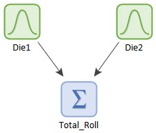
There are two Stochastic elements (one for each die), and a Sum element that simply adds their values together. Let’s look at Die1. Open it and press the Edit… button to view how the distribution is defined:
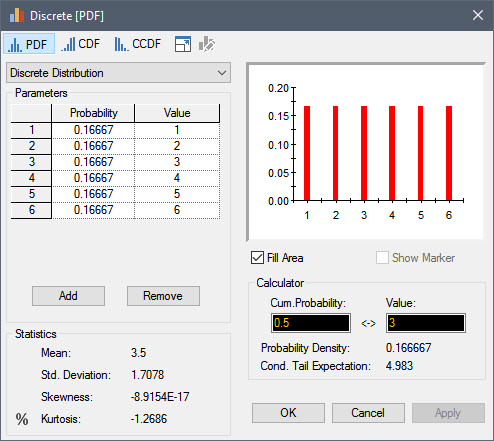
Recall from Lesson 3 that there are two kinds of distributions: discrete or continuous. Discrete distributions have a limited (discrete) number of possible values. Continuous distributions have an infinite number of possible values. Obviously, the probability distribution for the roll of a die is discrete: there are six and only six possible outcomes (you can’t roll a 3.5!). Each outcome is specified here as having an equal probability. Die2 is defined identically (in fact, after creating Die1, Die2 was created simply by cutting and pasting). Close this dialog (and the next) so we can look at the rest of the model.
Now that we see how the model is defined, let’s look at how the Monte Carlo settings have been defined. Monte Carlo options are defined using the Simulation Settings dialog. Recall that you can open the Simulation Settings dialog by pressing F2, choosing Run | Simulation Settings from the main menu bar, or by pressing Simulation Setting button in the toolbar:

Open the dialog now so we can examine it. This dialog has four tabs: Time, Monte Carlo, Globals and Information. For now, we are going to focus on the Monte Carlo tab:
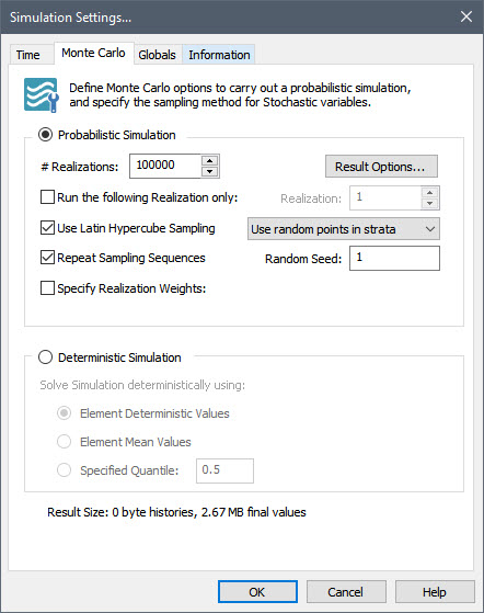
There are lots of options here, but the only one you need to notice right now is # Realizations. We have instructed GoldSim to run 100,000 realizations. That is, in terms of this model, we are going to simulate rolling the dice 100,000 times. (We will discuss some of the other options in the next Unit).
Before you close this dialog, return to the Time tab. You will note that the Time Basis is set to “Static Model” (in previous Examples and Exercises this has always been set to either “Elapsed Time” or “Calendar Time”). What does this mean? In this extremely simple model, nothing changes with time. All we are doing is rolling the dice and obtaining an answer. Each individual dice roll (i.e., each realization) is a “possible future” or “possible result”. As a result, for each realization we have simply told GoldSim to select a value for each of the Stochastic elements (we refer to this as “sampling” the distribution) and add them up for every realization (100,000 times). There is no reason to step through time within a realization (since the result every timestep for a given realization would be identical; once we roll the dice nothing happens). This is called a Static Model. Although in most cases, you will be running a dynamic model (“Elapsed Time” or “Calendar Time”) since you will be trying to predict how a system will evolve through time, occasionally when running Monte Carlo simulations for simple systems like this, you may want to run a Static Model as we have done here.
So let’s now close the Simulation Settings dialog and run the model. When we run a Monte Carlo simulation, what does GoldSim actually do?
- For realization #1, it randomly picks a value for each of the two Stochastics (based on the defined distribution). In this case, each random pick will have a 16.7% chance of being a 1, a 16.7% chance of being a 2, etc. This is referred to as sampling the distribution.
Note: You might be curious as to how GoldSim actually makes this “random pick” each realization for a particular Stochastic (i.e., how it “samples” the distribution). The mechanism by which GoldSim (and any Monte Carlo simulator) does this is conceptually straightforward, and involves using an algorithm that generates a string of random numbers (between 0 and 1). We will discuss this further in the next Unit.
- After sampling each Stochastic, it carries out the calculations for the model. In this example, that consists simply of adding them together using the Sum element.
- The results for that realization are saved.
- Steps #1 through #3 are then repeated for all realizations.
- At the end of the simulation, GoldSim has a set of n results (where n is the number of realizations). These results can be assembled into a probability distribution (in the same way that a frequency distribution can be created by tabulating and sorting multiple observations). In particular, in this simple case, GoldSim basically creates 11 different “bins” (one for each possible outcome), and simply keeps track of the number of realizations falling into each bin.
Note: This is obviously a simple case in that due to the nature of the model, there are a discrete number of possible results (11). That is, the output distribution is discrete. If at least one of the inputs (and hence the outputs) are continuous in nature, the approach is conceptually similar, with a larger number of “bins” being used to assemble the output distributions (in the extreme, one for each realization). If you are interested in these computational details (you probably aren’t!), they are described in Appendix B of the GoldSim User’s Guide.
Let’s look at the results now. What we are interested in is the Sum element (Total_Roll). Just like when viewing results for other models, right-clicking on the Sum element will provide a context menu for displaying results:
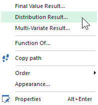
We are interested in viewing the output distribution (i.e., a probability distribution of the result), so we will select Distribution Result…
Note: In previous models that we have explored, when we right-clicked on an element in Result Mode there was another option: Time History Result… However, because this is a Static Model, this option is not available (there are no time histories to display).
Selecting Distribution Result… displays the following result dialog:
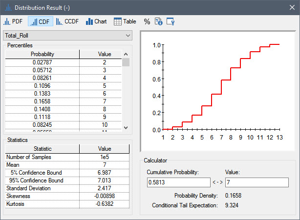
The first thing you will note is that this looks somewhat similar to the dialog used to define input probability distributions. But this is not an input; it is an output. This result display is expressing our uncertainty in the output (in this particular case, the output is the outcome of a role of two dice). The upper right-hand side of the dialog displays a plot of the result distribution. By default, it is displayed as a CDF (which is the most common way output distributions are presented). In this particular case, however, because the output distribution is discrete, this is not necessarily the most intuitive way to view the result. So let’s press the PDF button at the top of the dialog (in this case, we are actually telling GoldSim to display a PMF not a PDF). Now the display looks like this:
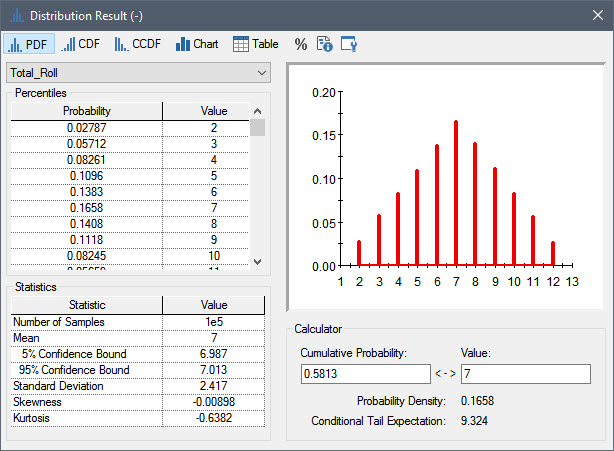
This plot should look familiar. It is similar to the result diagram shown in the previous Lesson showing the 36 combinations of dice rolls. Rather than generating the result by combinatorial analysis, however, we have generated it though Monte Carlo simulation. The left side of the dialog shows the probabilities displayed in the plot. Note that the probability for rolling a seven is reported to be 16.58%.
Note: When viewing a table like this, you can press Alt-Right and Alt-Left to display more or less significant figures.
Note: Because this result distribution is discrete, the table on the left side of this dialog shows probabilities. If the result was continuous, it would display percentiles. We’ll look at a continuous distribution result in Lesson 8.
In this simple case, we know (from the diagram at the beginning of this Lesson) that the actual probability is 16.67%. The accuracy of the Monte Carlo results increases with the number of realizations. As we do more and more realizations, this probability computed using Monte Carlo simulation would converge to the true probability. We will discuss this topic further in Lesson 8.
Pressing the Chart button displays a large plot of the distribution. Pressing the Chart button again then returns to the Result Summary dialog. Pressing the Table button displays a list of each of the 100,000 realizations:
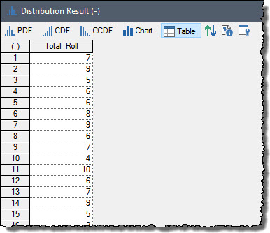
In this example, the first realization resulted in a roll of 7, the second was a 9, and so on. Pressing the Table button again then returns to the Result Summary dialog.
You can learn more about viewing distribution results like this in GoldSim Help.
Before closing this Example let’s address one additional topic. At the top of the dialog you will see the Edit Properties button:

Press this now and the following dialog will be displayed (the result display will not be closed, so that both dialogs will remain open):
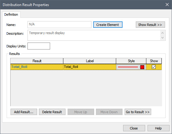
This dialog (and many of its features) are analogous to the properties dialog for a time history result. There are a number of things you can do with this dialog. Let’s highlight a few. First, note that you can change the Display Units (for the X-axis). It defaults to the Display Units that you used when you defined the element whose output is being viewed (in this case, the Sum element). You can change it here (in this example, however, the result is dimensionless so there would be no reason to do so). Note that changing the Display Units here does not change the units for the original element. It simply changes the units for the chart display.
The Add Result button allows you to add multiple outputs to the chart. For example, you could add each die separately, but we won’t bother to do so now.
You can change the line Style for the output. By default, the first line style that was added was red. Press the button under Style in the list. It will display the dialog that allows you to change the line style. Change it to blue and close the Style dialog. You could also change the Label. This column determines how the output is labeled in the chart legend and axes. By default, it is the name of the output. We can change that here. For example, since those names cannot have spaces, we needed to use an underscore in the element name. For the Label, remove that underscore now and replace it with a space.
After making such changes, close the Distribution Properties dialog (by pressing the Close button) and close the result display. Then view the result again (by right-clicking on the Sum, and selecting Distribution Result…). You will notice that all of the changes that were made (changing the view to PDF instead of CDF, changing the color, changing the label) have been lost!
What happened? Recall from our discussion on time history results that when you right-click on an element to view results, the result display itself is temporary. That is, the display is recreated every time your right-click and choose to view it. It is not saved by GoldSim (and hence none of the changes that you made are saved). Of course, if you are going to bother to makes such changes to a display, you want them to stick around. So how do we tell GoldSim to do that? We create a Result element. Just as we can create a Time History Result element, we can also create a Distribution Result element.
View the result again (by right-clicking on the Sum, and selecting Distribution Result…). Change the view to PDF, and then press the Edit Properties button to view the Distribution Properties. Make two minor changes (edit the Style to change the color to blue and remove the underscore from the Label). Now press the Create Element button at the top of the Properties dialog. When you do so, the dialog will change slightly to look like this:
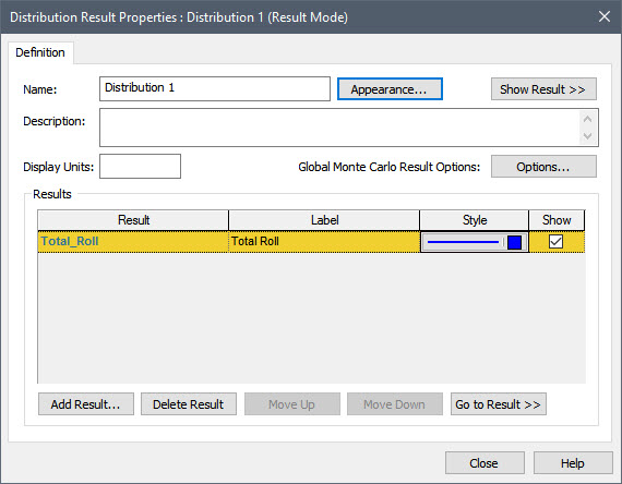
Note that you can now assign a Name to this element. And unlike other element names, this name can have spaces. Let’s change it to “Result”. Then close the dialog, and you will now see a new element in the graphics pane:

This is a Distribution Result element.
If you double-click on it (while in Result Mode), the Summary Result is displayed (preserving all of the formatting changes you have made). If you return to Edit Mode, re-run the model, and double-click on it again, the formatting is still there.
As we discussed when we introduced the Time History Result element (Unit 6, Lesson 12), Result elements are valuable for a number of reasons, including the following:
- They allow you to quickly display key results that you want to look at whenever you run the model and have been nicely formatted; and
- They allow you to view multiple results charts or tables simultaneously.