Courses: Introduction to GoldSim:
Unit 12 - Probabilistic Simulation: Part I
Lesson 4 - The Stochastic Element
Now that we have discussed how uncertainty is quantified using probability distributions, in this Lesson we will explore how probability distributions are actually defined within GoldSim.
Probability distributions are defined in GoldSim using the Stochastic element. Let’s insert and explore one now. You will find the Stochastic under the element category “Inputs”. You will see that the dialog for a Stochastic element looks like this:
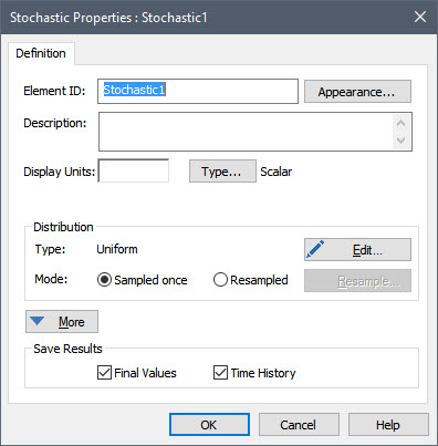
Like (almost) all elements, we first must specify an Element ID, Description and Display Units.
The Edit… button is used to define the probability distribution represented by this Stochastic element. Press that button now. The following dialog will be displayed:
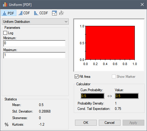
The drop-list in the upper left-hand corner of the dialog contains a list of all of the distributions provided by GoldSim. Directly below this field, you enter the parameters defining the selected distribution (the parameters differ depending on the distribution type). These can be constants, links to other outputs or expressions. Note that by default, it is defined as a Uniform distribution (which has two arguments, a Minimum and a Maximum). These default in a new element to 0 and 1, respectively. A plot of the distribution is displayed to the right.
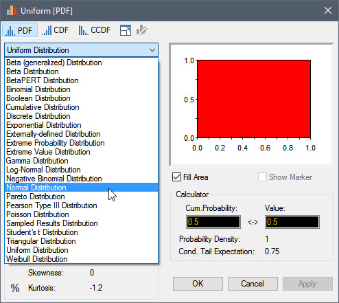
Let’s change the distribution now. Click on the drop-list and select “Normal”:
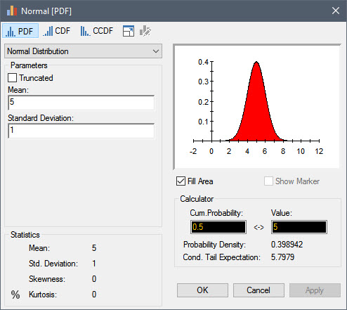
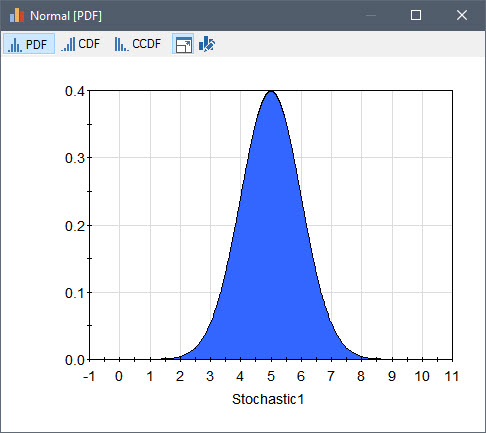
A Normal distribution requires a Mean and a Standard Deviation. Enter 5 and 1 for these, respectively. Then press the Apply button to update the plot of the distribution. (This plot is not updated until you press the Apply button or close and reopen the dialog). The dialog will now look like this:
By default, the distribution is displayed as a PDF. You can view it as a CDF or CCDF by pressing these buttons:
Now press the following button:

You will see that a large plot of the distribution is displayed:
Press the button again and you will return to the dialog for defining the distribution.
Directly below the section where you define the parameters for the distribution, various statistics for the distribution are displayed. In this section, you will see the percentile button:

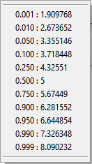
Press this button and the percentiles for the distribution will be displayed:
Click anywhere else and the percentiles list will close.
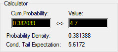
The Calculator section of the dialog allows you to compute the value associated with a particular percentile or the percentile associated with a particular value. For example, in the example below, by entering the value 4.7, we see that the percentile associated with this value is approximately 0.38:
Although we’ve covered all of the important points, if you wish you can read more about using this dialog in GoldSim Help.
Before leaving this dialog, you should spend some time selecting some of the other distribution types (and pressing the Apply button) to see what they look like. You can read about all of the distribution types (and how they are typically used) in GoldSim Help.
In Lesson 9 we will briefly discuss how specific distributions are chosen.
When you are done experimenting with distribution types, close the dialog and return to the main Stochastic element dialog.
Recall from the previous Lesson that we can use probability distributions to represent two different kinds of parameters: 1) those whose uncertainty is due to ignorance or lack of knowledge; and 2) those whose uncertainty is due to inherent randomness. We noted that we will actually treat them differently when we define these distributions within GoldSim. This is done using the two Mode radio buttons:
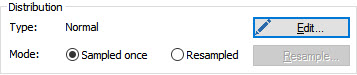
In particular, parameters whose uncertainty is due to ignorance or lack of knowledge are generally specified such that they have a constant value through time (“Sampled once”), while parameters whose uncertainty is due to inherent randomness are specified such that take on different values through time (“Resampled”).
For the remainder of this Unit, we will only deal with parameters whose uncertainty is due to ignorance or lack of knowledge, and will therefore use the default Mode setting (“Sampled once”). In Unit 13 we will discuss the “Resampled” setting.
Finally, you will note that the More button accesses several advanced options. We will discuss one of these later in this Unit.
Although we have learned how to create probability distributions, we have not learned how using them impacts our simulations. In the simplest terms, if the inputs to a model are uncertain, the outputs are also uncertain (i.e., they become probability distributions). In order for that to happen, however, we need to propagate the uncertainty in the inputs to the uncertainty in the outputs. We will discuss how GoldSim does that in the next Lesson.