Courses: Introduction to GoldSim:
Unit 12 - Probabilistic Simulation: Part I
Lesson 3 - Quantifying Uncertainty Using Probability Distributions
This Lesson is one of the most “theoretical” Lessons in this Course in that it describes a number of mathematical and subtle conceptual issues that may be new to some readers. Nevertheless, it is critical that you take the time to understand these concepts if you wish to carry out probabilistic analysis and take full advantage of GoldSim. Although these concepts may be new to many readers, as has been noted, they are not particularly complex and do not require any specialized knowledge.
In the previous Lesson, we discussed the concept of uncertainty. The natural question is then: “how do you represent and quantify these different types of uncertainty?” When uncertainty is quantified, it is expressed in terms of probability distributions. A probability distribution is a mathematical representation of the relative likelihood of a parameter having specific values.
There are a number of ways in which probability distributions can be graphically displayed. The simplest way is to express the distribution in terms of a probability density function (PDF). This plots the relative likelihood of the various possible values, and is illustrated schematically below:
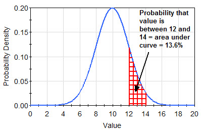
Note that the “height” of the PDF for any given value is not a direct measurement of the probability of the corresponding value. Rather, it represents the probability density. The units of a probability density are the inverse of the units of the parameter. The total area under the PDF integrates to 1.0. Therefore, integrating under the PDF between any two points results in the probability of the value being between those two points.
There are many types of probability distributions. Simple distributions include the normal, uniform and triangular distributions, illustrated below:
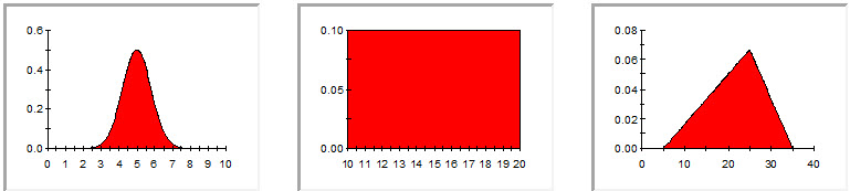
All distribution types use a set of arguments to specify the relative likelihood for each possible value. For example, the normal distribution uses a mean and a standard deviation as its arguments. The mean defines the value around which the bell curve will be centered, and the standard deviation defines the spread of values around the mean. The arguments for a uniform distribution are a minimum and a maximum value. The arguments for a triangular distribution are a minimum value, a most likely value, and a maximum value.
The nature of an uncertain parameter, and hence the form of the associated probability distribution, can be either discrete or continuous. Discrete distributions have a discrete (and for practical purposes, limited) number of possible values (e.g., 0 or 1; yes or no; 10, 20, or 30). Continuous distributions have an infinite number of possible values (e.g., the normal, uniform and triangular distributions shown above are continuous). Two examples of discrete distributions are shown below:
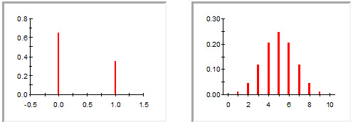
Note: Discrete distributions are actually described mathematically using probability mass functions (PMF), rather than probability density functions. Probability mass functions specify actual probabilities for given values, rather than probability densities.
Although PMFs are easy to interpret and use, PDFs are actually more difficult to use since the y-axis represents a probability density (which is a rather abstract concept).
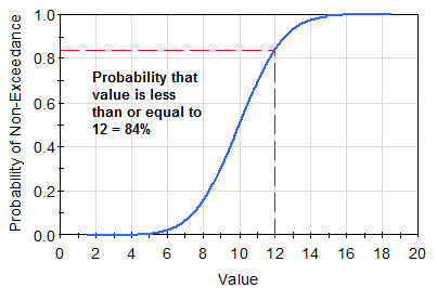
Hence, an alternative manner of representing the same information contained in a PDF (or a PMF), particularly when viewing probabilistic results (as opposed to specifying inputs), is the cumulative distribution function (CDF). This is created by integrating the PDF. Since the total area under the PDF integrates to 1.0, the CDF therefore ranges from 0.0 to 1.0.
For any value on the horizontal axis, the CDF shows the cumulative probability that the variable is less than or equal to that value. That is, as shown below, a particular point, say [12, 0.84], on the CDF is interpreted as follows: the probability that the value is less than or equal to 12 is equal to 0.84 (84%).
A third manner of presenting this information is the complementary cumulative distribution function (CCDF). The CCDF is illustrated schematically below:
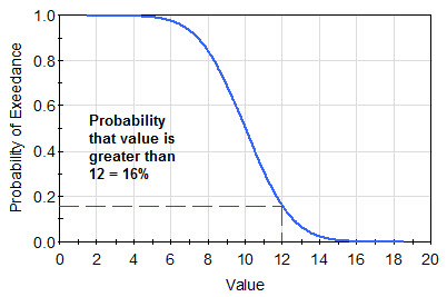
A particular point, say [12, 0.16], on the CCDF is interpreted as follows: the probability that the value is greater than 12 is 0.16 (16%). Note that the CCDF is simply the complement of the CDF; that is, in this example 0.84 is equal to 1 – 0.16.
Probability distributions are often described using percentiles of the CDF. Percentiles of a distribution divide the total frequency of occurrence into hundredths. For example, the 90th percentile is that value of the parameter below which 90% of the distribution lies. The 50th percentile is referred to as the median.
Of course, when building models, you will need to decide the appropriate distribution to use for any given uncertain parameter. We will discuss this in some detail in Lesson 9. As we will see in a subsequent Lesson, GoldSim provides a specialized element for specifying probability distributions (and viewing them as a PDF/PMF, CDF or CCDF).
Let’s return now to the two types of uncertainty described in the previous Lesson. Both types of uncertainty can be represented using probability distributions. However, as we noted, we need to be careful to understand that they are representing different things.
Uncertainty due to lack of knowledge can be represented using a probability distribution, with the “spread” (e.g., standard deviation) of the distribution representing the degree of our uncertainty (the “wider” the distribution, the poorer our knowledge). If we were to study the parameter, our knowledge theoretically would increase such that the distribution should become “narrower” (i.e., the standard deviation should become smaller).
Parameters that are inherently random can also be represented using probability distributions. In this case, however, these are more correctly referred to as frequency distributions. A frequency distribution displays the relative frequency of a particular value versus the value. For example, one could sample the flow rate of a river once every hour for a week, and create a frequency distribution of the hourly flow rate (the x-axis being the flow rate, and the y-axis being a measure of the frequency of the observation over the week). Note, however, that once you have made such measurements, studying such a parameter further does not reduce the standard deviation of the distribution, since the shape of the distribution is inherent to the nature of the parameter: it is randomly variable (although of course it may also have an underlying trend).
As we shall see in the next Lesson, because these two types of uncertainty are conceptually different, we will actually treat them differently when we define these distributions within GoldSim. In particular, we will see that parameters whose uncertainty is due to lack of knowledge will be specified such that they have a single constant value through time, while parameters whose uncertainty is due to inherent randomness will be specified such that they take on different values through time.
As we pointed out in the previous Lesson, some parameters exhibit both types of uncertainty. Representing this in a probability distribution must be done with care: in particular, we should not simply lump both types of uncertainty together. So how could you represent such a parameter? As an example, consider the flow rate in a river. We know that it will be temporally variable (inherently random), but if we have not taken a lot of measurements, we may have uncertainty about the statistical measures (e.g., mean, standard deviation) describing that variability. To represent this properly in GoldSim we would first define a frequency distribution that represented the inherent temporal variability of the parameter. Having done so, the arguments for the frequency distribution itself (e.g., mean and standard deviation) would themselves be defined as probability distributions (to represent our lack of knowledge).
Note: For dealing with problems where both types of uncertainty are important, GoldSim provides an advanced analysis feature (referred to as nested Monte Carlo) that can be used to explicitly represent and evaluate these uncertainties in a detailed manner. This advanced feature, however, is beyond the scope of this Course.
It turns out that in practice, although some parameters do indeed exhibit both types of uncertainty, one type often dominates (and hence is the only one that is represented). As a result, in this Course, we will only consider parameters that exhibit one type of uncertainty or the other.
Before leaving this topic, there is one additional point that is important to make, as a lack of understanding of this point is a common source of errors in probabilistic simulations. In the discussion above, we have described two different kinds of parameters that can be represented in probabilistic simulations using probability distributions:
- Parameters which are uncertain due to a lack of knowledge. These have a single (actual) constant value, but we don’t know enough to determine that single value, and hence must represent it as a probability distribution that represents our lack of knowledge.
- Parameters whose uncertainty is due to inherent randomness. These are inherently variable (random or noisy) over time such that their behavior can only be described statistically. The probability (actually, frequency) distribution represents this variability.
Those of you with a statistical background may notice that there is actually a third kind of parameter (that we have not discussed) that can also be described using a distribution. In particular, many quantities are variable not over time, but over space or within a collection of items or instances, and we can also describe this variability using a probability (actually, frequency) distribution. An example is the size distribution of a collection of marbles. If you had a collection of 1000 marbles, you could measure the size of each marble and create a frequency distribution of the size of the marbles in the collection. This kind of distribution is similar to that discussed in the second bullet above (inherent randomness, in which a parameter changes with time) in that both are described using frequency distributions (one showing a frequency in time, and one showing a frequency of occurrence within a group).
With regard to making predictions using simulation, however, the marble example is fundamentally different from an inherently random (time-variable) parameter. Whereas a distribution representing an inherently random parameter truly is describing uncertainty (we are inherently uncertain about its value at any given time and hence are unable to precisely predict the value at any given time in the future), a distribution representing the variability in marble size is not describing uncertainty (i.e., unpredictability) at all. It is simply describing variability within the group that we could actually measure and define very precisely if we needed to in order to make predictions about the behavior of each of the marbles.
Similar to when we were describing the need to separate inherent randomness from lack of knowledge earlier in this Lesson, it is critical to separate variability like this from uncertainty when representing this in GoldSim. This is particularly important, as it is very common for parameters to be both uncertain and variable (in space or across a group). For example, suppose that you needed to represent the efficacy of a new drug for which the efficacy is different for different age groups (in this example, the distribution of ages is conceptually similar to the distribution of marble sizes discussed above). Moreover, for each age group, there exists scientific uncertainty regarding its efficacy. A common mistake would be to define a single probability distribution for the efficacy that “lumps together” both the variability in the efficacy due to age and the uncertainty in the efficacy (which might actually differ for each age group). Not only would it be difficult to define the shape of such a distribution in the first place, but this would produce simulation results that would be difficult, if not impossible, to interpret and use in a meaningful way. The correct way to handle such a situation would be to disaggregate the problem (by explicitly modeling each age group separately) and then define different probability distributions for the efficacy for each age group (with each distribution representing only the scientific uncertainty in the efficacy for that age group). Because this is one of the common mistakes when defining probability distributions, we will discuss it again in Lesson 9.