Courses: Introduction to GoldSim:
Unit 12 - Probabilistic Simulation: Part I
Lesson 5 - Propagating Uncertainty Using Monte Carlo Simulation
If the inputs describing a system are uncertain, the prediction of the future performance of the system is necessarily uncertain. That is, the result of any analysis based on inputs represented by probability distributions is itself a probability distribution.
In order to compute the probability distribution of predicted simulation results, it is necessary to propagate (translate) the input uncertainties into uncertainties in the results. A variety of methods exist for propagating uncertainty. The most common (and most flexible) technique for propagating the uncertainty in the inputs to the uncertainty in the outputs (and the one used by GoldSim) is Monte Carlo simulation.
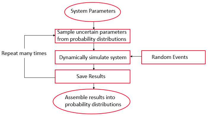
In a Monte Carlo simulation, the entire system is simulated a large number (e.g., 1000) of times. By default, each simulation is equally likely, and is referred to as a realization of the system. For each realization, a random value for all of the uncertain parameters described by probability distributions is selected (based on the distribution). The system is then simulated through time (given that particular set of input parameters) such that the outputs of the system can be computed.
This results in a large number of separate and independent results, each representing a possible “future” for the system (i.e., one possible path the system may follow through time). The results of the independent realizations are assembled into probability distributions of possible outcomes. A schematic of the Monte Carlo method is shown below:
As a simple example of a Monte Carlo simulation, let’s assume that the uncertain result we want to calculate is the probability of a particular sum of the throw of two dice (with each die having values one through six). For each die, we are uncertain what its roll will be (if the die is fair, there is an equal probability of any of six values). It turns out that in this particular case (because it is quite simple), we can manually propagate the uncertainty using combinatorial analysis. That is, we can tabulate the 36 combinations of dice rolls:
Based on this, we can manually compute the probability of a particular outcome. For example, there are six different ways that the dice could sum to seven. Hence, the probability of rolling seven is equal to 6 divided by 36 = 0.167.
Instead of computing the probability in this way, however, we could instead throw the dice a thousand times and record how many times each outcome occurs. If the dice totaled seven 171 times (out of 1000 rolls), we would conclude that the probability of rolling seven is approximately 0.171 (17.1%). Obviously, the more times we rolled the dice, the less approximate our result would be. Doing so constitutes a Monte Carlo simulation (and we did not even need a computer!).
Of course, rather than rolling the dice a thousand times, we can much more easily use a computer to simulate rolling the dice 1000 times (or more). Because we know the probability of a particular outcome for one die (1 in 6 for all six numbers), this is simple. In fact, in the next Lesson, we will use GoldSim to do exactly that.
Note: As you can imagine, running a complex model for a large number of realizations can become computationally intensive. Fortunately, Monte Carlo simulation lends itself to parallel processing (since each realization is independent of the others). This means that conceptually, you can run each realization on a different processor (or computer) and then combine the results together. In fact, although it is rarely necessary, GoldSim provides the ability to easily do this (and we will discuss that briefly in Unit 18).
As an interesting aside, you might be interested to know that Monte Carlo simulation is named after the city in Monaco (famous for its casino) where games of chance (e.g., roulette, craps) involve repetitive events with known probabilities. Although there were a number of isolated and undeveloped applications of Monte Carlo simulation principles at earlier dates, modern application of Monte Carlo methods date from the 1940s during work on the atomic bomb. Mathematician Stanislaw Ulam is credited with recognizing how computers could make Monte Carlo simulations of complex systems feasible:
"The first thoughts and attempts I made to practice [the Monte Carlo Method] were suggested by a question which occurred to me in 1946 as I was … playing solitaires. The question was what are the chances that a Canfield solitaire laid out with 52 cards will come out successfully? After spending a lot of time trying to estimate them by pure combinatorial calculations, I wondered whether a more practical method than “abstract thinking” might not be to lay it out say one hundred times and simply observe and count the number of successful plays. This was already possible to envisage with the beginning of the new era of fast computers... Later … [in 1946, I] described the idea to John von Neumann, and we began to plan actual calculations."
Eckhardt, Roger (1987). “Stan Ulam, John von Neumann, and the Monte Carlo method”, Los Alamos Science, Special Issue (15), 131-137