Courses: The GoldSim Contaminant Transport Module:
Unit 2 - Using Arrays in GoldSim
Lesson 9 – Exercise: Creating and Viewing Probabilistic Vector Results
In this Lesson we will carry out an Exercise that produces probabilistic results for a vector.
Note: It is assumed here that you are familiar with probabilistic modeling in GoldSim (as discussed in Unit 12 and Unit 13 of the Basic GoldSim Course).
We are going to start with the model we built in the previous Exercise. You should have saved that model and named it ExerciseCT1.gsm (in the “MyModels” subfolder of the “Contaminant Transport Course” folder). Open the model now. (If you failed to save that model, you can find the Exercise, named ExerciseCT1_Vectors.gsm, in the “Exercises” subfolder of the “Contaminant Transport Course” folder you should have downloaded and unzipped to your Desktop.)
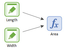
You will recall that in that model we defined the Length and Width for our fields (using vectors), and then carried out a number of calculations on those. Delete all of the elements for the calculations except the one that computed the Area of each field, so your model should look like this:
Let’s assume that a farmer is going to irrigate each of these fields at a particular rate (in mm/day) for the next 100 days. Each field is irrigated at a fixed rate. But for a variety of reasons (e.g., equipment issues) there is day to day random variability in the rate for each field that, based on past measurements, can be described statistically. That is, the daily variability can be described by specifying the irrigation rate for each field using a frequency distribution:
| Field | Irrigation Rate (mm/day) |
|---|---|
| North | Truncated Normal(20 mm/day, 5 mm/day, Minimum 0 mm/day) |
| South | Exponential(10 mm/day) |
| East | Truncated Normal(50 mm/day, 10 mm/day, Minimum 0 mm/day) |
| West | Exponential(12 mm/day) |
That is, the North and East fields can be described using a Normal distribution (with a specified mean and standard deviation), and the South and West fields can be described using an Exponential distribution (with a specified mean). The two Normal distributions are truncated at zero because a negative rate is not physically possible (but could occur if we did not truncate the distribution).
Note: In GoldSim, you will need to define these using Stochastic elements that are resampled every day. Resampling Stochastics is discussed Unit 13, Lesson 2 of the Basic GoldSim Course.
What we would like to do is calculate the cumulative volume of water (in m3) applied to each field over the 100-day period. Because the inputs are stochastic, this result will be a probability distribution, so we want to display the distributions for all four fields. To do so, let’s run the model for 100 realizations.
The first thing you will need to do is to build a vector of probability distributions for the irrigation rates. You should do so by first creating scalar Stochastic elements representing the rate for each field, and then combining these into a vector of irrigation rates (we will talk about why this is the only way to do this below). You should then 1) convert the irrigation rates to volumetric rates (by multiplying by the Area), and 2) use a Reservoir element to accumulate the volumetric rates to compute the total volume applied over 100 days.
Stop now and try to build the model.
If, and only if, you get stuck, open and look at the worked out Exercise (ExerciseCT2_Probabilistic.gsm in the “Exercises” subfolder) to help you finish the model.
Let’s walk through the model now.
You may have been tempted to define the four irrigation rates using a single Stochastic element (Stochastic elements can be defined as vectors). If you tried to do so, however, you would have discovered that it is not possible. This is why it was noted above that you should instead create four scalar elements first and then combine them. Let’s take a minute to discuss that before we continue.
You can indeed create a Stochastic element and define it as a vector (of fields in this case), as shown below:
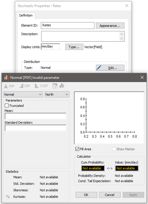
However, if you do this, all items of the vector must be defined using the same distribution type (in the example above, a Normal). In this case, the inputs (e.g., mean and standard deviation) must be vectors. In some situations, you might be able to do this. Often, however, and in particular in our Exercise, the four items do not have the same distribution type. Hence, this approach will not work.
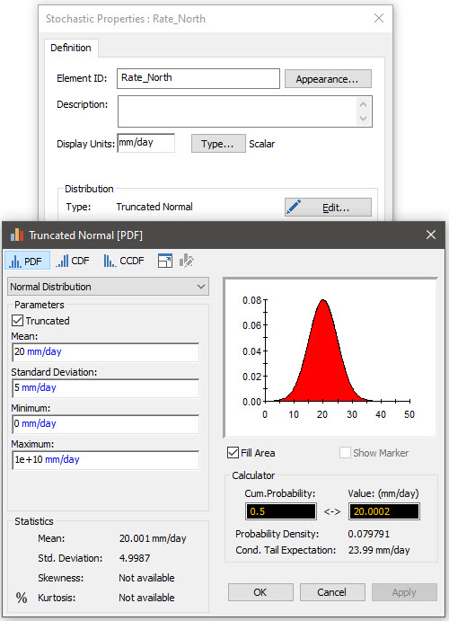
Instead, we must define each distribution separately as a scalar (in this case, requiring four Stochastic elements). For example, here is the Stochastic element representing the North field:
Once all four Stochastics are defined, we next need to combine them into a vector. As we learned in earlier Lessons, there are two ways to do this. One would be to use a vector constructor function in an Expression that looked like this:
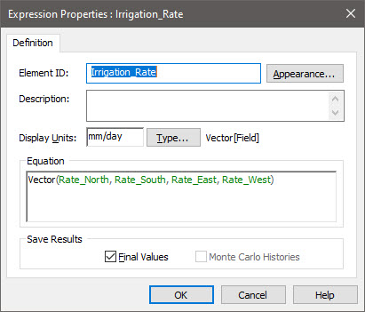
Although this would work in this simple Exercise (since there are only 4 items in the vector), if there were many items in the vector, it would be awkward. As a result, a better way to build this vector is to use a Data element:
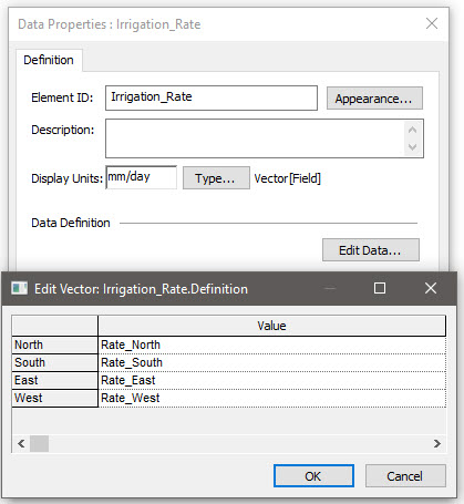
This provides a very easy to understand way to build a vector from a collection of scalar outputs.
Note: As a general rule, Data elements should not contain links like we have done here (as it defeats the purpose of the visual cue provided by the element icon that indicates that this is data as opposed to a link or equation). In fact, this was specifically discussed in Unit 5, Lesson 6 of the Basic GoldSim Course. However, this is the one exception to that rule. Stylistically, Data elements can contain links if they are being used to construct arrays from a collection of scalar outputs.
Note: This example is not here by accident. As we will see in later Units, many inputs for the Contaminant Transport Module will be vectors (of the different contaminant species being simulated). Moreover, many of these inputs will be uncertain and hence represented by different probability distributions. As a result, it would not be uncommon to use a similar structure to what we have done here (building a vector of probability distributions using a Data element) to represent these vector inputs.
We can now compute the volumetric rate by multiplying the irrigation rate by the area for each field:

Finally, we can accumulate that rate by using a Reservoir:
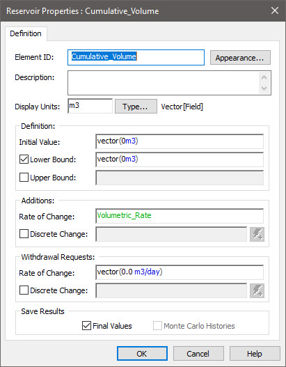
Note that all the inputs to the Reservoir must themselves be vectors.
If we run the model for 100 days, and then right-click on the Reservoir and select Distribution Result… we see this:
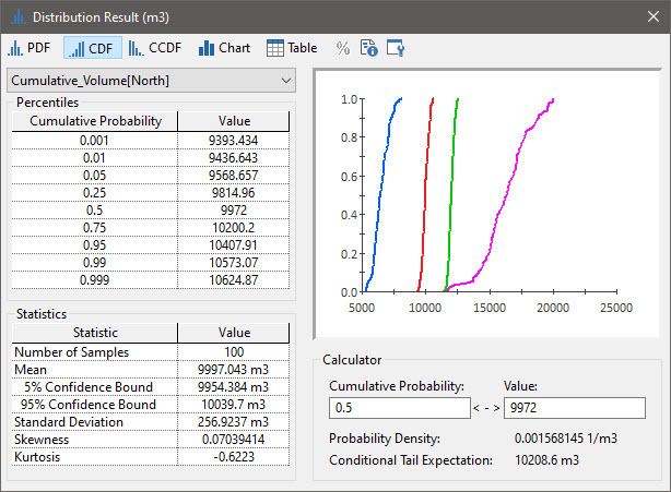
Viewing a Distribution result for an array is treated as if you are viewing a Distribution result for multiple outputs.
The Preview Pane on the right shows all four results (in this case, the four vector items). The Percentiles and Statistics obviously can only be shown for one item at a time (and this is selected from the drop-list at the top).
Note: The completed Exercise provided in the Exercises subfolder includes a Distribution Result element in which the labels and axis titles have been modified from their defaults.
As shown in the previous Lesson, we can also plot a time history of the Cumulative Volume. To do so, however, we would have to create a Time History Result element that referenced the Reservoir prior to running the model. Since we have multiple things to plot (i.e., each item) and multiple realizations, the chart and table result windows provide multiple options for viewing the results. In the example below, the 100th realization is plotted for all four items:
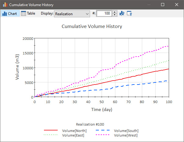
We could also plot various statistics (e.g., the mean for each item).