Lesson 8 - Referencing Vectors in Other GoldSim Elements and Viewing Vector Results

In the previous Lessons we discussed how vectors can be created and manipulated using mathematical operators and built-in functions. In addition, it is important to understand that many of the GoldSim elements can manipulate (and output) arrays. For example, you can add a number of vectors using the Sum element, or compute the peak value of each item of a vector using the Extrema element. Other elements such as Stochastics and Reservoirs can also be vectors.

To illustrate this, let’s walk through a very simple example together. Select File|Open… from the main menu in GoldSim.  It will open a Windows browser.  Browse to the “Contaminant Transport Course” folder on your Desktop that you unzipped, and inside that folder you will find another folder named “Examples”.  Inside that folder will be a file named ExampleCT1_Evaporating_Ponds.gsm.  Select that file to open it.  The model looks like this:

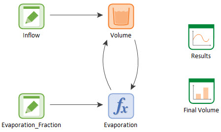
This is actually a slightly modified version of an Exercise from the Basic GoldSim Course (Unit 8, Lesson 4). That original model simulated a pond (that starts empty), has a constant inflow rate of water, but also evaporates.  The evaporation rate is simply assumed to be proportional to the volume. This example model is identical to that original model with one difference: instead of modeling a single pond, we are modeling three ponds, and are doing so by using vectors.

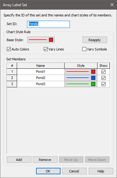
To do so, we created an Array Label set named Ponds.  You can view it by selecting Model|Array Labels from the main menu and double-clicking on the Ponds set:

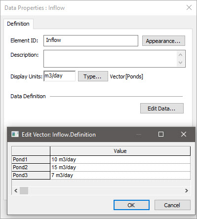
In the model, Inflow, Evaporation and Volume are all vectors of Ponds (Evaporation_Fraction is a scalar). Inflow is defined as follows:

Volume (a Reservoir element) looks like this:

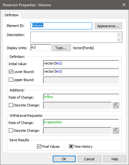
Since the Reservoir is defined as a vector, all of its inputs must also be vectors.  The outputs of the Reservoir are then vectors.  The Reservoir’s calculations are simply carried out in parallel for each item of the vector.

To view a time history of results, the primary output of the Reservoir has been added to a Time History Result element. Double-click on the Time History Result element to view the Properties dialog:

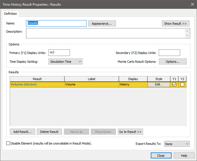
As can be seen, the output is added to the Result element as a single result (and it is indicated that this is a vector).  Close the dialog, run the model and double-click on the Time History Result element:

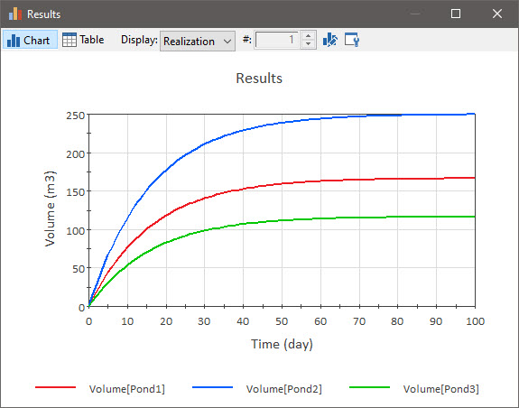
Note that all three items of the vector are shown in the chart.

Now return to Edit Mode (by pressing F4) and double-click on the element named Final Volume:

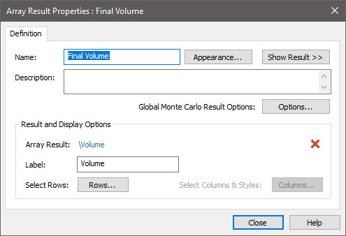
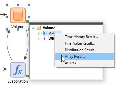
This is an Array result. Array results allow you to view “snapshots” of arrays at particular points in time in both graphical and tabular form. By default, this is at the end of the realization (the final values). This is an Array Result element.  You can also view array results by selecting Array Result… from the context menu for the result (by left-clicking on the output port and then right-clicking on the result of interest):

Close the dialog, run the model and double-click on the Array Result element:

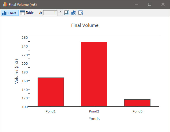
As you can see, the final values for the three items of the array are displayed in the form of a bar chart

Note: You can also produce a similar chart using a Final Value Result.  Final Value Results were introduced and discussion in Unit 7, Lesson 8 or the Basic Course.

In the next Lesson we will work on another Exercise that explores a few additional features of manipulating vectors and displaying vector results.