Courses: Introduction to GoldSim:
Unit 11 - Dealing with Dates and Time
Lesson 5 - Defining Time Series
In the previous Lesson, we built a simple example showing how we could make a variable (in this case, an evaporation rate) vary by season. In particular, we made it vary by calendar month by referencing the Month Run Property. This allowed us to model a seasonal trend that repeated every year (recall that the evaporation rate was the same every year for a particular month). Of course, we could have added a longer term trend (up or down) to the Expression, and as we will discuss in the next Unit, we could also have added some random variability. However, the key point is that we created an expression (an equation) that described how the variable changed with time.
In many cases, however, you will want to input external time histories of data into your models; that is, a table showing how a variable will change throughout the simulation (e.g., every hour, every day). Such a table of data is referred to as a time series. When you enter a time series as an input, you are explicitly specifying how a variable will change with time during the simulation. That is, you are stating that the way it will change is actually known in advance (or, more commonly, simply assumed to behave in a certain way for the purpose of the simulation). As such, a time series represents an exogenous (external) influence on the evolution of a model (Unit 6, Lesson 2).
Some examples of time series inputs include the following:
- The rainfall rate in a model predicting the future volume of water in a pond or lake.
- The immigration rate of people into a region in a model used to predict demand for water, food or some other resource.
- The price of a commodity in a business model for a company that must purchase (or sell) that commodity.
- The sales rate of a product in a business model for a company.
In all of these cases, you should only specify a time series as an input if you can reasonably assume that the input itself is truly exogenous (i.e., the model itself has no impact on the input). This would certainly be the case for a model simulating the volume of water in a lake – that volume is highly unlikely to have any effect on the rainfall rate. However, it is less likely to be true (over the long term) for the second example listed above – at some point, if the demand for the resource increases, the immigration rate may decrease due to the lack of the resource (i.e., there is a feedback loop between the demand and the immigration rate). Similarly, in the third example, the behavior of the company could in fact feedback on (and affect) the price of the commodity, and in the fourth example, the behavior of the company could feedback on (and affect) the sales rate. On the other hand, depending on the scope of the system and the model, it may in fact be completely appropriate to treat these last three examples as exogenous inputs that are unaffected by the model itself.
Note: This brief discussion brings up a critical point that must be carefully considered in ALL models: what is the “boundary” of the model? Anything outside the boundary is unaffected by anything inside the boundary (and hence can be considered exogenous). A very common error in many simulation models is to incorrectly define the boundary (i.e., assume a variable is exogenous, and hence can be specified directly, when it actually is influenced to some extent by variables inside the model).
Having discussed what a time series is, let’s now discuss how we would create one in GoldSim. Conceptually, a time series could simply be considered a 1-D Lookup Table in which the independent variable is time. Although this is true, practically it would be difficult to use a Lookup Table in this way for a variety of reasons (e.g., Lookup Tables cannot handle dates). Moreover, that is not really what Lookup Tables were intended for. They are response surfaces (i.e., user-defined functions).
As a result, GoldSim provides a special element (the Time Series element) that is specifically designed to define time series inputs. To understand how a Time Series element works, let’s open a new model and insert and explore one now. You will find the Time Series under the element category “Inputs”. You will see that the dialog for a Time Series element looks like this:
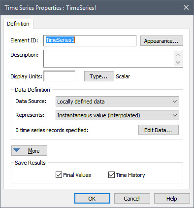
The dialog for the Time Series element is actually one of the more complex element dialogs in GoldSim (the More button provides a variety of advanced options). For now, however, we don’t need to worry about the advanced options, and can just focus on the basic fields.
First notice the Data Source field. This is where you specify where the time series data is coming from. It can be entered directly (“Locally defined data”, the default), or can be imported from a spreadsheet. (There are also some advanced options here that we will not discuss). For now, we will enter the data locally, so there is no need to change anything here.
Before we enter any data however (via the Edit Data button), let’s define the Display Units. In this little example, we are going to be specifying a sales rate, so let’s define the Display Units as $/day. After doing so, press the Edit Data button. The following dialog will be displayed:
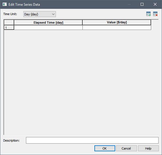
Note that there are two columns here. The first is time, and the second is the value of the time series itself (at that time point). By default, there is a single (empty) row. You can add (and remove) rows using the buttons in the upper right-hand corner of the dialog:

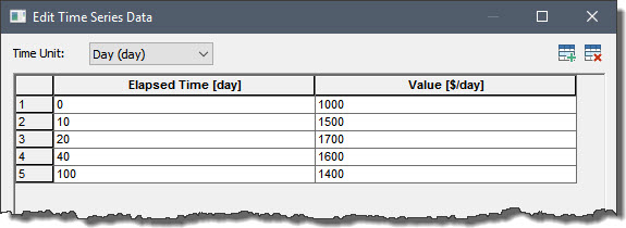
Add four more rows so we have a total of 5 empty rows, then enter some data so it looks like this:
Note: When you enter data into a Time Series element, you can only enter numbers (you cannot enter links to other elements). Note also that you do not append units to the values; the units are indicated in the header.
Note: The values of time must increase monotonically as you move downward in the table. If they do not, GoldSim will automatically resort the rows into the correct order when you close the dialog.
Note: In most cases, when using Time Series you would enter a large number of rows (hundreds or thousands). As such, you would almost never enter the data manually like we did here. We will discuss importing data from a spreadsheet in a subsequent Lesson.
How exactly will GoldSim interpret this Time Series? For example, we have specified a value at 40 days and at 100 days, but what then is the value in between these points? The best way to start to understand this is to simply run the model and see what the Time Series outputs.
If we run the model, and then right-click on the Time Series element to view its time history, it looks like this (note that by default the model runs for 100 days with a 1 day timestep):
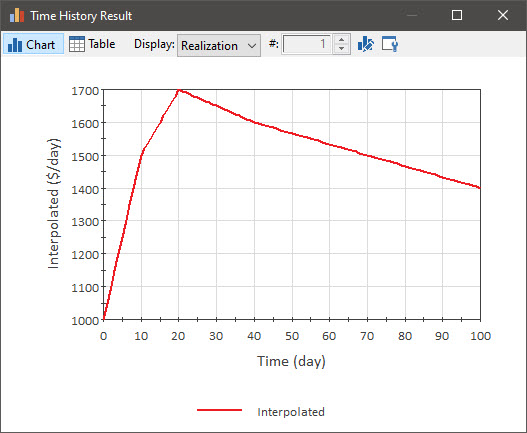
What should be apparent here is that for the values in between the specified time points, GoldSim has interpolated values. So, for example, at time 30 days (halfway between data points at 20 days and 40 days), the value is assumed to be 1650 $/day (halfway between the values at those two points).
But is that what was really intended? Perhaps. But in other cases, we may have wanted to interpret the data differently. In fact, GoldSim specifically requires you to specify how you want to interpret the data, and it is critical to specify this appropriately. Return to Edit Mode and look at the Time Series dialog again. You will notice a field named Represents. This is where you specify how you would like GoldSim to interpret the data. You will note that there are a number of choices:
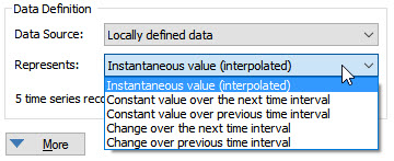
For now, however, let’s just focus on the first three. The first option (and the default) is “Instantaneous value (interpolated)”. In this case, we are telling GoldSim that each time point represents an instantaneous measurement at that point in time. Hence, the most appropriate thing to do between time points is to interpolate. Examples of such data would include the price of a stock or commodity, or the height of a projectile. In our simple example, this was the default option, so GoldSim interpolated.
Often it is inappropriate, however, to interpolate between data points, and instead more appropriate to assume that a value is constant over a specified interval. In some cases, it may actually physically be constant; in others this may simply be an artifact of how the data was recorded (e.g., it may have only been recorded as an average value over an interval). In such a case, it would be inappropriate to interpolate between the data points. GoldSim provides two options for representing this kind of data (one is forward-looking and one is backward-looking): “Constant value over the next time interval” and “Constant value over the previous time interval”.
To understand how these work, let’s edit our simple example as follows:
- Rename the existing Time Series to “Interpolated”.
- Copy it and paste it, and rename the new Time Series to “ConstantOverNext”.
- Open the second Time Series and change Represents to “Constant value over the next time interval”.
- Copy the “ConstantOverNext” element and paste it, and rename the new Time Series to “ConstantOverPrevious”.
- Open the second Time Series and change Represents to “Constant value over the previous time interval”.
- Rerun the model and plot all three on the same chart. It will look like this:
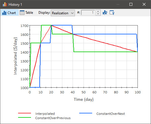
If the data represents “Constant value over the next time interval”, given a particular time point/data pair (e.g., 20 days; 1700 $/day), the value provided at that point is assumed to be the value from the current time point to the next time point (e.g., the value is held at 1700 $/day between 20 and 40 days). If the data represents “Constant value over the previous time interval”, given a particular time point/data pair (e.g., 20 days; 1700 $/day) the value provided at that point is assumed to be the value from the previous time point to the current time point (e.g., the value is held at 1700 $/day between 10 and 20 days).
Note that all three Time Series use the exact same data. The only thing that is different is how the data is to be interpreted (i.e., what it Represents). Clearly, the results can be quite different. Hence, when entering such time series data, it is important that you think carefully about how the data was collected and exactly what it represents. Should it be interpolated between points? Should it be held constant between points? If so, is the data forward-looking or backward-looking?
GoldSim provides several other (advanced) options for how to interpret the data, and you can read about the details of these various options in GoldSim Help.
The simple example discussed above defined the time series in terms of elapsed time. Time Series elements, however, are much more frequently used in calendar-based models, in which case the time series is defined in terms of dates, rather than elapsed times. This is because the reason for using a time series is often to represent things in which the month or hour of day is important (i.e., to represent seasonal or diurnal trends).
Time Series elements support this by allowing you to enter your data points on a calendar basis. We can see this by looking at the simple example we have been discussing, and returning to Edit Mode. Open one of the Time Series elements and view the data again. You will note that at the top of the dialog, you can specify the Time Unit:
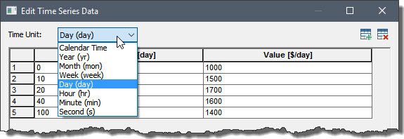
The default is (elapsed) days. In fact, all but the first option are for specifying time in terms of different units of elapsed time. The first option (“Calendar time”) allows you to enter data in terms of dates/times. Select it now and note what happens to the values:
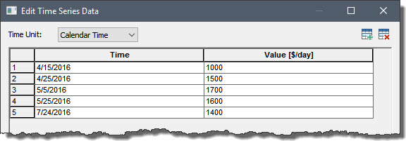
GoldSim displays the time in terms of dates (your dates will be different; GoldSim converts from elapsed time based on the Start Time in your simulation settings).
In addition to entering dates, you could also specify times using this format: MM/DD/YYYY HH:MM:SS (the date format is determined by the Windows Regional Settings on your computer).
There are many more advanced Time Series features that we have not discussed (the Time Series element is quite complex), but the basics that we have covered here are sufficient for the purposes of this Course. If you want to learn more about some of the advanced Time Series features, consult GoldSim Help.
In the next several Lessons, we will build some models using some of the basic Time Series features we have discussed here.