Courses: Introduction to GoldSim:
Unit 11 - Dealing with Dates and Time
Lesson 7 - Using Historic Data in a Time Series Element
In most cases, you will want to use historic data to populate a time series. For example, you might have decades of daily rainfall records, commodity prices or temperature. In such a case, of course, you would not enter the data by hand. One option would be to paste directly into the data table from a spreadsheet, Word table, or comma-delimited text file (by clicking in the cell representing the upper left-hand corner of the region of the table into which you wish to paste, and pressing Ctrl+V).
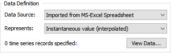
Alternatively, you can tell GoldSim to import the data directly from a spreadsheet. To do so, you need to specify the Data Source as “Imported from MS-Excel Spreadsheet”:
When you do so, a new tab (Excel) is added to the dialog that allows you to define the properties of the spreadsheet link:
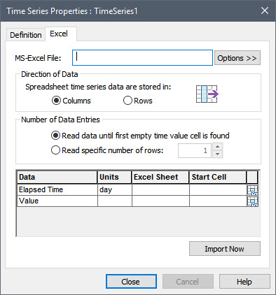
We will use this tab and explore the options further in an Exercise in the next Lesson.
Of course, when we import historic data, it will be imported using calendar-based times (from the past). But most simulations look forward in time (i.e., we build simulations to predict what will happen in the future). For example, if we had 20 years of daily temperature data (e.g., from 1990 to 2010), and wanted to use this data in a 2 year simulation (e.g., from 2017 to 2019), how would we do that? In the simulation, the Time Series would need to specify the values from 2017 to 2019 (not 1990 to 2010). Obviously, in order to use this data, we need to shift it. That is, we need to shift the data from historic dates to other dates (e.g., assume 2017 will be identical to 1990).
To support this, GoldSim provides an option to time shift the data in a specified manner. This feature is provided in the “Advanced” section of the Time Series dialog, accessed via the More button. To explore this a bit further, let’s look at a pre-built model. You will find this model in the “Examples” subfolder of the “Basic GoldSim Course” folder you should have downloaded and unzipped to your Desktop. In that folder, open a model file named Example17_TimeShifting.gsm.
This is a very simple model consisting of a single Time Series element. If you explore the model, you will note the following:
- In the Simulation Settings dialog you will see that the simulation is set to run for 10 years (1/1/2017 to 1/1/2027), with a 1 day timestep.
- The Time Series represents daily flow rates in a river from 1923 to 2010 (there are almost 32,000 data points!). The units are in “cfs” – cubic feet per second.
You will note that in the Time Series dialog, the dialog has been extended and the “Advanced” section is visible (this section becomes visible by pressing the More button, and if some advanced options have been selected cannot be hidden). The “Advanced” section looks like this:
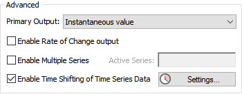
You will note that the box next to Enable Time Shifting of Time Series Data is selected (this is why the Advanced section is visible and cannot be hidden). Press the Settings… button next to this field and the following dialog will appear:
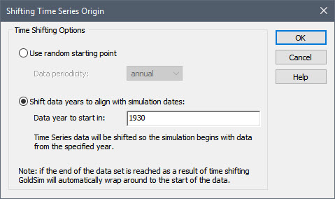
This dialog allows you to define how the data is to be time shifted. GoldSim provides two different ways that Time Series can be shifted.
The first option is to Use random starting point. This option randomly samples a starting point in the data set for each realization. This is useful, for example, if you have 50 years of rainfall data, you want to carry out a 1 year simulation, and you want to run a probabilistic simulation and randomly sample a different historic year for each realization. We will revisit this option in Unit 13.
The second option for time shifting the Time Series is to Shift data years to align with simulation dates. This option shifts the time series data such that the simulation begins by mapping data from the specified Data year to start in to the simulation Start Time.
In this example, the Data year to start in is set to 1930. Recall that the simulation Start Time was 1 January 2017. As a result, GoldSim treats the data set such that the data point corresponding to 1 January 1930 would be used for 1 January 2017 (and, because daily data was entered, the data point for 2 January 1930 would be used for 2 January 2017, etc.). Because this is a 10 year simulation, what this means is that the period from January 2017 to January 2027 will be assumed to behave exactly like the historic period from January 1930 to January 1940.
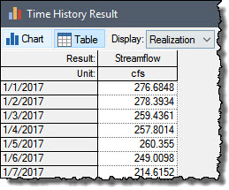
To verify this behavior, open the Time Series, press Edit Data, and find the value corresponding to 1 January 1930. You will note that it is 276.6848. Now run the model, right-click on the element to view time histories, and press the Table button to view a table of results (as opposed to a plot). You will see that the first data point (at 1 January 2017) is indeed 276.6848:
Note: When viewing the table, you can press Alt-Right and Alt-Left to display more or less significant figures.
Note: What if the Data year to start in was set to a year at the end of the data set (e.g., 2008) such that there were not 10 subsequent years to use? In that case, GoldSim “wraps” the data around and returns to the start of the data set. That is, it would use 2008, 2009 and 2010, and then wrap around back to 1923 for additional data to complete the 10 years of simulated time.
You can read more about time shifting Time Series elements in GoldSim Help.
In the next Lesson, we will work though an Exercise in which we import data from a spreadsheet and time shift it.