Courses: Introduction to GoldSim:
Unit 11 - Dealing with Dates and Time
Lesson 8 - Exercise: Modeling Seasonal Variables in a Time Series Element
Now that we have learned the basics of importing time series data from a spreadsheet and subsequently time shifting that data, let’s do an Exercise to actually carry out those operations.
We are going to start with a new model, so you can create a new model now. We are going to do the following:
- In Simulation Settings, set up a Calendar Time run with Start Time 1/1/2017 and End Time 1/1/2027, with a 1 day timestep.
- Insert a Time Series element, and name it Rainfall. Give it Display Units of mm/day.
- Specify that the Data Source is “Imported from MS-Excel Spreadsheet”. When you do this, an Excel tab will appear.
- We are going to import the rainfall data from a spreadsheet. You will find the spreadsheet we are going to use in the “Exercises” subfolder of the “Basic GoldSim Course” folder you should have downloaded and unzipped to your Desktop. The name of the spreadsheet is Exercise16_Data.xlsx. Open the spreadsheet file and you will notice that it contains two columns of data. Make sure you close the spreadsheet before proceeding.
- In the Excel tab of the Time Series, see if you can figure out how to import the data from the spreadsheet. You may want to refer to GoldSim Help if you get stuck.
- Next go back to the main Time Series dialog and press the More button to expand the dialog.
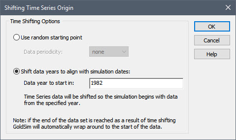
- Activate time shifting by checking the box for Enable Time Shifting of Time Series Data, and press the Settings button. Then select the radio button for Shift data years to to align with simulation dates, and enter a Data year to start in of 1982.
- Run the model and plot a time history of the Time Series.
Stop now and try to build and run the model.
Once you are done with your model, save it to the “MyModels” subfolder of the “Basic GoldSim Course” folder on your desktop (call it Exercise16.gsm). If, and only if, you get stuck, open and look at the worked out Exercise (Exercise16_ TimeSeries_Shift.gsm in the “Exercises” subfolder) to help you finish the model.
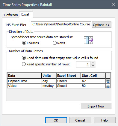
In case you had problems importing the data, let’s walk through those steps right now. The Excel tab looks like this:
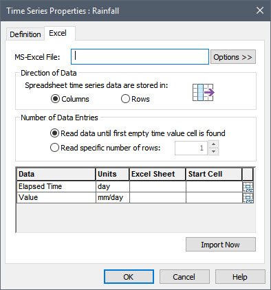
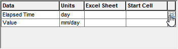
The first thing you need to do is specify the spreadsheet. You do this by pressing the Options>> button, selecting “Select existing MS-Excel file…”, and browsing to the spreadsheet and selecting it. For the next two fields, we can stick to the default options (“Columns” and “Read data until first empty time value cell is found”). Next we need to specify where in the spreadsheet the data is stored. The easiest way to do this is to press the Link button in the time row:
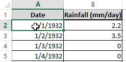
When you do this, it will open the spreadsheet. Select the cell containing the first date (in this case A2):
You will note a small dialog titled “GoldSim – Excel Location Selection”:
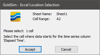
Press the Accept button. When you do so, GoldSim will insert the Sheet and Start Cell information. Press Import Now and GoldSim will import the data. After doing so, the Excel tab will look like this:
If you return to the main dialog, you will note that 29221 data points were imported. You can press View Data to view the imported data. You will note that it starts on 1/1/1932 and goes through 1/1/2012.
Setting up the time shifting is straightforward. The Shifting Time Series Origin dialog should look like this:
If we then run the model and plot a time history of the Time Series, it should look like this:
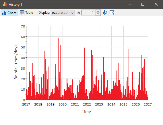
Note the seasonal trend in the rainfall.
Note: Whenever your run a model in which the Data Source is set to “Imported from MS-Excel Spreadsheet”, GoldSim will import the data every time the model is run. Although this is useful if you will subsequently modify the spreadsheet, it is not necessary if you have no plans to do so. In that case, after you import the data, you should return to the main tab and set the Data Source back to “Locally defined data”. The Time Series will no longer be linked to the spreadsheet, but all of the data that was previously imported will remain.