Courses: Introduction to GoldSim:
Unit 11 - Dealing with Dates and Time
Lesson 6 - Exercise: Using a Time Series Element to Specify a Time-Varying Input
Now that we have learned the basics of Time Series elements, let’s do an Exercise to get a bit more comfortable with them.
We are going to start with a model we built in a previous Exercise. You should have saved a model named Exercise3.gsm. Open the model now. (If you failed to save that model, you can find the Exercise, named Exercise3_Selector_Runoff.gsm, in the “Exercises” subfolder of the “Basic GoldSim Course” folder you should have downloaded and unzipped to your Desktop.)
Open that model and refresh your memory on what we did in that simple model. Recall that we calculated the volumetric runoff rate (volume/time) during a rainfall event and then calculated the cumulative volume of water that ran off over a 48 hour period (by using a Reservoir). The rainfall rate was assumed to vary with time. In particular, we assumed the following:
- Rain does not begin falling until after 10 days, at which time it falls at 60 mm/day.
- At 15 days, the rainfall rate doubles to 120 mm/day.
- At 20 days, it stops raining.
We ran the model for 50 days and plotted the accumulated the runoff.
In that model, we represented the rainfall rate using a Selector element. You may recall that at the time we noted that there is actually a much better way to implement this without using a Selector (but it provided a quick way to illustrate the use of a Selector). You should be able to see now that a Time Series element provides a much easier and more transparent way to represent the rainfall.
In this Exercise, we are simply going to replace the Selector (and any inputs it references) with a Time Series element.
Stop now and try to build the model.
Once you are done with your model, save it to the “MyModels” subfolder of the “Basic GoldSim Course” folder on your desktop (call it Exercise15.gsm). If, and only if, you get stuck, open and look at the worked out Exercise (Exercise15_ TimeSeries_Runoff.gsm in the “Exercises” subfolder) to help you finish the model.
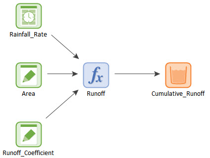
Your new model structure should look something like this (the Selector and any elements that it references have been deleted and replaced with a Time Series element):
The Time Series element is defined as follows:
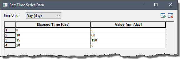
Importantly, the Represents field should be “Constant value over the next time interval”.
Now open up the Time History Result element. When you do so, you will note that the second item is invalid (it is displayed in red). This is because we just replaced it (it used to be a Selector, now it is a Time Series). Simply click on the Result "Rainfall_Rate" and select it again from the dialog and it will become valid again.
If you run the model and plot the cumulative runoff, the result will look like this (which is identical to the result using a Selector):
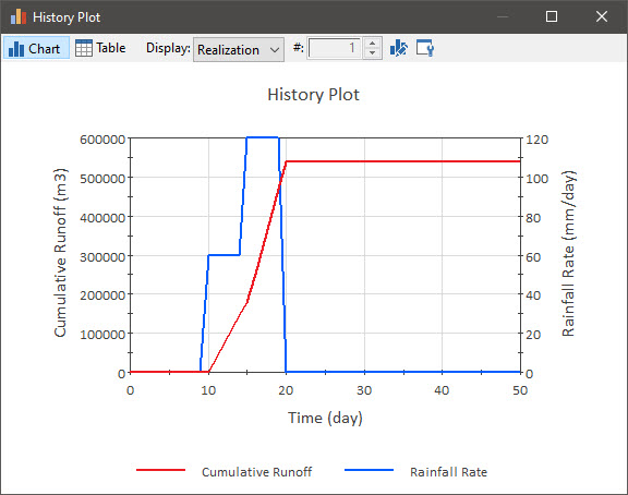
Clearly, using a Time Series to represent the rainfall rate is much simpler (both to enter and understand) than using a Selector.