Courses: Introduction to GoldSim:
Unit 11 - Dealing with Dates and Time
Lesson 9 - Using Reporting Periods
In many cases (particularly when running calendar-based models) you may have a short timestep (e.g., daily), but want to report results (e.g., average values) over longer specified periods (e.g., monthly, annually). For example, perhaps you were simulating the growth rate of a population using a monthly timestep, but wanted to report the average annual growth rate each year. Or perhaps you were simulating the flow rate in a river using a daily timestep, but wanted to report the monthly and annual average flow rates.
To support this, GoldSim allows you to create Reporting Periods. The best way to understand and explore Reporting Periods is to experiment with a model. Let’s use the same Example model that we looked at in Lesson 7. You will find this model in the “Examples” subfolder of the “Basic GoldSim Course” folder you should have downloaded and unzipped to your Desktop. In that folder open a model file named Example17_TimeShifting.gsm.
As you may recall, this is a very simple model consisting of a single Time Series element. The simulation is set to run for 10 years (1/1/2017 to 1/1/2027), with a 1 day timestep. The Time Series represents daily flow rates in a river from 1923 to 2010. The data was shifted such that the Data year to start in is set to 1930.
Let’s open up the Simulation Settings and set up some Reporting Periods:
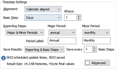
Make the changes you see here. In particular:
- Set Reporting Steps to “Major & Minor Periods”. The two Periods will default to “annual” and “monthly”.
- The Period Labels will default to “Major” and “Minor”. Change the Period Labels to “Annual” for the Major Period and “Monthly” for the Minor Period.
- Set Save Results to “Reporting & Basic Steps”; and
- Set Save Every to 1.
What we have done is set up two Reporting Periods and told GoldSim to not only save results at the end of each Reporting Period, but to also save all of the Basic Steps (this will allow us to better understand the results).
So now that we have set up Reporting Periods, how do we view them in results? It turns out that Reporting Period results can only be defined and viewed via Time History Result elements. That is, the act of creating Reporting Periods does not in itself provide specialized Reporting Period-based results. To display specialized Reporting Period-based results, you must add the outputs you are interested in to a Time History Result element, and then specify that you want to view Reporting Period-based results. Let’s do that now.
Make sure you are in Edit Mode, and insert a Time History Result element (it can be found under the “Results” category). Press the Add Result… button and add the Time Series element. The dialog should then look like this:
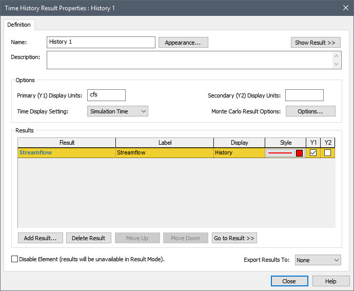
Note that by default, the Time Display Setting in this dialog is set to “Simulation Time”. In this case, Time History results simply provide instantaneous values at each saved timestep. Since we have defined Reporting Periods, however, we can change the Time Display Setting to “Reporting Periods”. When we do so, the dialog is changed:
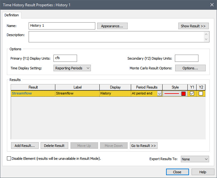
In particular, a new column is added (Period Results). This is a drop-list that allows you to select results based on Reporting Periods. There are six options. We won’t explore them all here (we will just consider three). If you are interested, you can read about them all in detail in GoldSim Help.
The default option is “At period end”. Let’s change this to “All plot points”. This displays instantaneous values at all the plot points (scheduled updates). This would include not only values at the end of each Reporting Period, but also values at all other scheduled updates (e.g., Basic Steps). This display is identical to what you would see if you selected “Simulation Time” for the Time Display Settings. Hence, it is not very interesting (as we are not taking advantage of Reporting Periods yet).
Now press the Add Result… button and add the Time Series element again. So you will have two rows, each of which has the Time Series specified as the Result. For this second row, however, specify the Period Results as “Average”. Then change the Label for the first row to “Flow” and the Label for the second row to “Average Flow”:
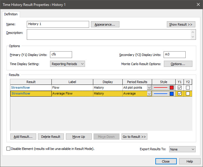
So when we run this model, we expect to see two lines: 1) one showing the instantaneous results at all plot points (in this case, every day); and 2) one showing values averaged (annually or monthly).
Now run the model and double-click on the Time History Result element to display the result:
Note: Your plot will have a Header (displaying the name of the Time History Result element). You can hide this by right-clicking in the plot, selecting View from the menu, and clearing the check next to “Show Header”.
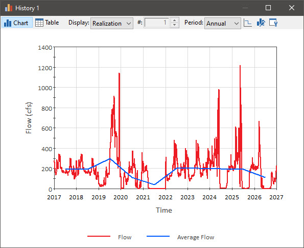
The red line shows the instantaneous flow rate (each day). The green line shows the average flow rate over the selected Reporting Period (in this case, the annual average).
By default, the Reporting Period Average is plotted as a line connecting the mid-point of each period (you will note that in the plot above, this is the mid-point of each year). How the Average is plotted is controlled by this button at the top of the display window:
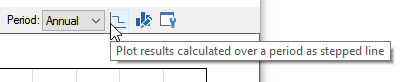
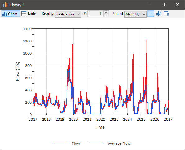
If the button is pressed, the Average is plotted as a stair-step (showing a constant value for each period). Press the button now. The result will now look like this:

Recall that we actually created two Reporting Periods: Annual and Monthly. Which is shown is controlled by the Period drop list at the top of the display window. We have been looking at “Annual” results. Use this drop list to select “Monthly”:
If you press the Table button, you can see a table view of the data:
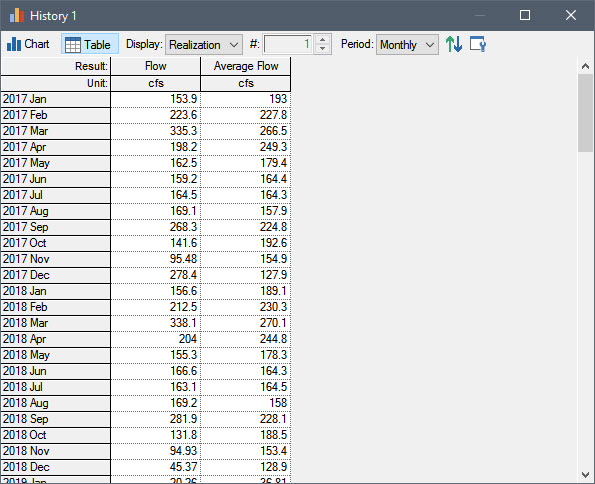
As can be seen, the results are only shown for each reporting period (in this example, each month). In this case, the “Average Flow” is the monthly average. In a table view, “Flow” (which you recall in the Chart was plotted for every plot point) represents the instantaneous value at the end of the Reporting Period.
Note: Recall (from Unit 6, Lesson 13) that you can use a Time History Result element to export results to a spreadsheet. When you export results that are Reporting Period-based, and you have two Reporting Periods defined, you must specify which Reporting Period to use during the export.
Before we leave the discussion of Reporting Periods, let’s quickly look at one more option for Period Results. Return to Edit Mode and open the Result element again. Select the second row, and press the Add Result… button and add the Time Series element again (i.e., a third time). (Selecting the second row first ensures that the new row is added below the second row). So you will now have three rows, each of which has the Time Series specified as the Result. For the new (third) row, specify the Period Results as “Cumulative”. Then change the Label for the third row to “Cumulative Volume”:
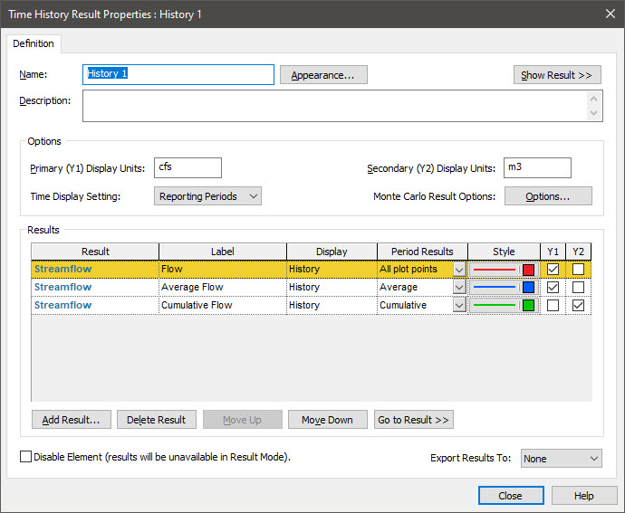
Note that the Y2 box is checked next to the third row. This output actually has different dimensions than the first two (and hence must be plotted on the other Y-axis). This is because this Period Result computes the integral of the value over each Reporting Period (from the end of the previous Reporting Period to the end of the current Reporting Period). As a result, it has dimensions of X*Time, where X is the dimensions of the actual output. Since X in this example is a volumetric flow rate, the dimensions of the Cumulative Period Result are a volume. In particular, it represents the quantity (i.e., the volume) that flowed (or accumulated) over each Reporting Period. Before we leave this dialog, we need to specify the units in which we want the Time History Result to display this result (Secondary (Y2) Display Units). It defaults to the display units of the primary axis multiplied by the Time Display Units (from the Simulation Settings dialog). Hence, in this case, it is cfs-day, which is a strange unit! So let’s change it to m3.
Now run the model and double-click on the Time History Result element. Select “Annual” (rather than “Monthly”) for the Period, and press the third button from the left at the top of the window so the results are plotted as a line connecting the mid-point of each period (rather than a stair-step). The result should look like this:
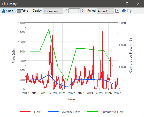
Note that the cumulative flow (the green line) is plotted using the Y2 (right-hand) axis.
We are going to revisit this example again in the next Lesson, so since we have changed it, save it to the “MyModels” subfolder of the “Basic GoldSim Course” folder on your desktop (call it Example18_TimeShifting_with_Reporting_Periods.gsm).