Courses: Introduction to GoldSim:
Unit 13 - Probabilistic Simulation: Part II
Lesson 10 - Viewing Distribution Results at Different Times in a Simulation
In this Lesson, we are going to revisit the display of distribution results (discussed in detail Unit 12). To do so, we are going to re-examine one of the examples we looked at in that Unit. Go to the “Examples” subfolder of the “Basic GoldSim Course” folder you should have downloaded and unzipped to your Desktop, and open a model file named Example20_UncertainEvaporation.gsm.
We looked at this model in Unit 12, Lesson 7. This is a model of an evaporating pond with an uncertain inflow rate.
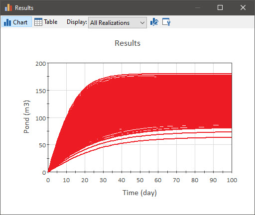
If you run the model, open the Time History Result element and then select “All Realizations” from the Display drop-list, the results look like this:
An alternative way for displaying multiple realizations is to show probability histories (by selecting “Probabilities” from the Display drop-list):
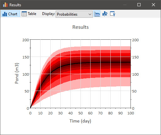
Recall that in a probability histories display, multiple realizations are representing by displaying the percentiles (as well as the bounds and the mean) of the set of time histories (each color band represents a different percentile region which you can identify by either right-clicking on the plot and showing the legend, or using the cursor to display a tool-tip).
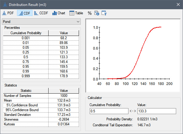
Distribution results essentially plot a vertical slice through this particular view. By default, the slice you get is at the end of the simulation (in this case, 100 days). So if you right-click on the Pond element and select Distribution Result… GoldSim displays the distribution of the final value of the pond volume:
However, what if we wanted to view a distribution of results at some other time in the simulation (instead of only at the end)? GoldSim facilitates this by allowing you to create Capture Times at which these results are also made available.
Capture Times are defined in the Advanced Time Settings dialog. You can access this by going to the Time tab of the Simulation Settings dialog and pressing the Advanced… button (make sure you are in Edit Mode and do that now). The top of the Advanced Time Settings dialog looks like this:
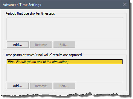
The second section from the top is where you define Capture Times. Note that there is always a Capture Time at the end of the simulation (which cannot be deleted). You can add a new Capture Time by pressing the Add… button. Let’s do that now. The following dialog will be displayed:
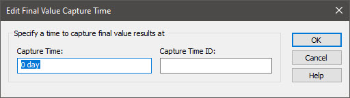
Let’s specify a Capture Time of 10 days. When creating a Capture Time, you must provide it with a Capture Time ID, which is used as a label when accessing Capture Time results in various result displays. Let’s name this one “Ten Days”.
Note: If you were running a Calendar Time simulation, you would enter a date for the Capture Time rather than an elapsed time.
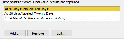
Now add another Capture Time at 20 days:

When you are done, the dialog should look like this:
Close the dialog (and the Simulation Settings dialog) and rerun the model. Now right-click on the Pond element and select Distribution Result…
What you should note is that there is a Time drop-list that allows you to select which “slice” you want to display:
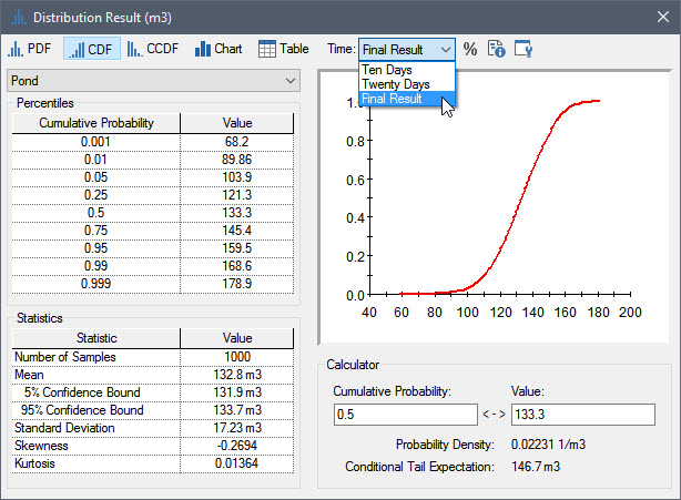
By default, it will be the “Final Value”, but you can choose one of the other two options also. Do that now to see how the display changes. When you are done, you can close this model.