Courses: Introduction to GoldSim:
Unit 13 - Probabilistic Simulation: Part II
Lesson 9 - Classifying and Screening Realizations
When carrying out probabilistic simulations, you may run hundreds or thousands of realizations. In order to analyze the results, it is often quite useful to classify the realizations into categories. A category is simply defined by a condition relating one or more outputs in the model (e.g., those realizations in which the discount rate was above 3.5%; those realizations in which the profit exceeded $1,000,000; those realizations in which the peak concentration was between 1 mg/l and 10 mg/l).
The power of categories is that once you have defined them, you can use them in two ways:
- Within certain kinds of result charts (e.g., scatter plots, time histories, distributions), realizations from each category can be displayed in a different color (and/or symbol).
- Within all result displays, you can choose to screen out one or more categories, so that the results that are shown (in charts and tables) only include those realizations in the categories which you have chosen to include.
The easiest way to illustrate this is to look at a simple Example. To do so, go to the “Examples” subfolder of the “GoldSim Course” folder you should have downloaded and unzipped to your Desktop, and open a model file named Example23_Categories.gsm.
The model looks like this:
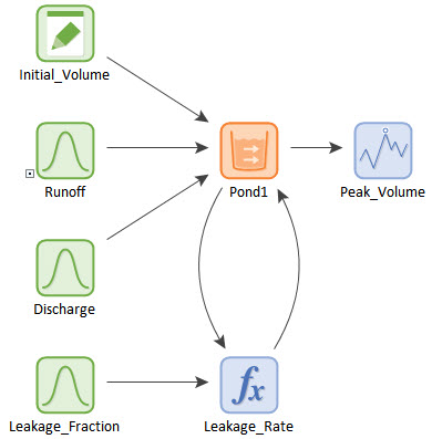
Runoff and Discharge are inflows into a pond. Runoff varies stochastically (it is resampled every day), and Discharge is simply an uncertain variable (it is sampled once each realization). The pond leaks, and the leakage rate is proportional to the pond volume (with the constant of proportionality being Leakage_Fraction). The Leakage_Fraction is also an uncertain variable (it is sampled once each realization). We are also using an Extrema to compute the peak pond volume.
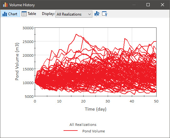
If you run this model for 100 realizations and view a time history of the pond volume (the Time History Result element named Volume History), the result looks like this:
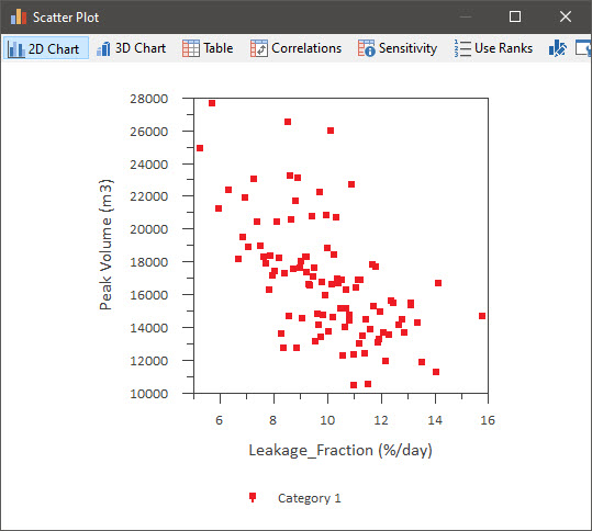
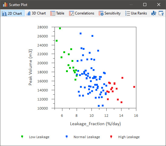
In order to analyze these results and better understand the behavior, it would be of value to see how the Leakage_Fraction impacts the results. Of course, as discussed in the previous Unit (Unit 12, Lesson 10) one way to do that would be to simply view a scatter plot of the peak pond volume versus the Leakage_Fraction (the Multi-Variate Result element named Scatter Plot):
We could also view Correlations for these variables.
What might be interesting to do, however, would be to examine how the Leakage_Rate affects the time history display. We can do this by defining some result categories. To do that, remain in Result Mode (you can do this from Edit Mode too, but it is somewhat more instructive to do it from Result Mode) and do the following:
- Open the Simulation Settings dialog and select the Monte Carlo tab.
- Press the Result Options… dialog and the following dialog will be displayed:
Note: As we shall see shortly, this dialog is also accessible from Result Properties dialogs.
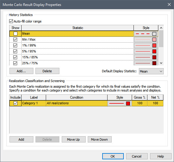
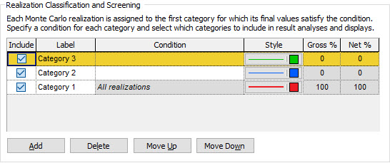
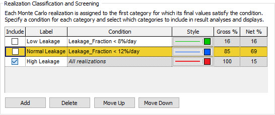
We are going to focus on the bottom portion of the dialog (“Realization Classification and Screening”). This is where we can classify all of the realizations into different categories. By default, all results are placed in a single category (defined as “All realizations”).
You can add categories by pressing the Add button. When you do so, it adds a row above the selected row. For each category that you add, you must define a Label and a Condition. Let’s add some categories now. Press the Add button twice. This will insert two new categories:
We now need to define the Condition for the two categories:
- For the first category in the list, define the Condition as: Leakage_Fraction < 8%/day. Change the Label to: Low Leakage.
- For the second category in the list, define the Condition as: Leakage_Fraction < 12%/day. Change the Label to: Normal Leakage.
- For the final category in the list, change the Label to: High Leakage.
The dialog should look like this:
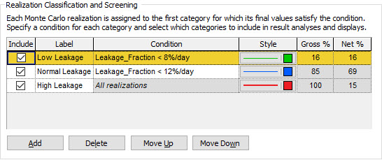
So what have we done here? We defined a category (named Low Leakage) that consists of all realizations in which Leakage_Fraction < 8%/day. As can be seen, 16 of the 100 realizations fall into this category. Next, we defined a category (named Normal Leakage) that consists of all the remaining realizations in which Leakage_Fraction < 12%/day. As can be seen, 69 of the 100 realizations fall into this category. Finally, we defined a category (named High Leakage) that consists of all the remaining realizations. Based on our definitions for the previous two categories, this would consist of all realizations in which Leakage_Fraction >= 12%/day. As can be seen, 15 of the 100 realizations fall into this category. The key point here is that the order of the categories is important. If multiple categories are true for a realization, the realization is assigned to the category with the first True Condition in the list.
So now that we have defined these categories, how can we use them? Close the dialogs and return to the GoldSim graphics pane. Let’s look at the Volume History Result element again:
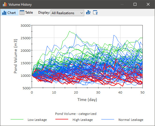
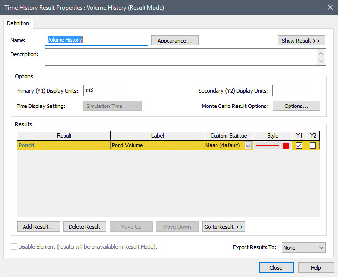
Note that the different categories are now identified (by color) in the time history chart. We can see, for example, that most of the high pond volume histories correspond to the Low Leakage category (as we would expect). Now press the Edit Properties button:

The Result Properties dialog will appear:
If you press the Options… button here, you can access the Monte Carlo Result Display Properties dialog (which we previously accessed via the Monte Carlo tab of the Simulation Settings dialog).
At the bottom of that dialog, let’s screen the realizations in the Low and Normal categories by clearing their Include boxes:
After doing so, close the dialog and view the Time History Result again:
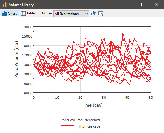
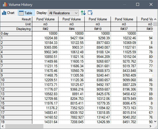
You will see that only the 15 High Leakage realizations are shown. If you press the Table button to view a table display of the result, again only those 15 realizations are included:
This can be very useful for “zooming in” on just those time histories of particular interest.
Before closing the Time History Result, press the Edit Properties button again and select Options… to access the Monte Carlo Result Display Properties dialog again. Then turn the two categories that we just turned off back on (i.e., make sure the Include boxes are checked for all three categories).
Now close the Time History Result element and instead let’s look at the Scatter Plot Result element:
This particular plot is not very interesting, as the variable on the x-axis is also the one that is color coded (i.e., the one used to define the categories). Let’s change that by pressing the Edit Properties button to access the Result Properties page:
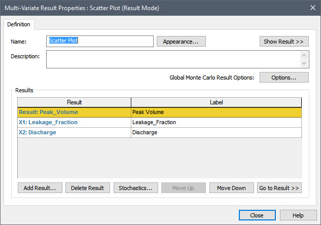
Select the third row (Discharge) and press the Move Up button to make it the x-axis. The Scatter Plot will now look like this:
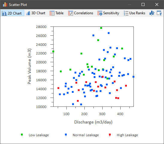
This helps us to visualize the results a bit more clearly. And like the case for time history results, if you wished, you could screen one or more of the categories from the result display if you wished.
You can also apply categories to distribution results, but we won’t take the time to do that now. If you are interested, you can read more in GoldSim Help.