Courses: Introduction to GoldSim:
Unit 13 - Probabilistic Simulation: Part II
Lesson 3 - Exercise: Stochastic Inflow
Now that we know how to create a Stochastic element that is resampled instead of sampled only once, let’s do a physically-based Exercise in which we simulate a stochastic process.
We are going to start with an Exercise we built in the previous Unit. You should have saved a model named Exercise17.gsm. Open the model now. (If you failed to save that model, you can find the Exercise, named Exercise17_Overflow_Uncertain.gsm, in the “Exercises” subfolder of the “Basic GoldSim Course” folder you should have downloaded and unzipped to your Desktop.)
Open that file and refresh your memory on what we did in that simple model. Recall that this model simulated a pond that received an inflow. The pond has an Upper Bound, and when the volume reaches that level it overflows into two other ponds (70% to one and 30% to the other).
Note: Recall that this model was originally built using Reservoirs for the stocks of material (water) instead of Pools (as we had not yet introduced Pools). If we were to build this model from the beginning again, it would be best practice to use Pools, as they are more powerful and flexible for material management problems (although in this case, that extra power and flexibility is not required). Since the model already exists, however, we will continue to use Reservoirs for the stocks.
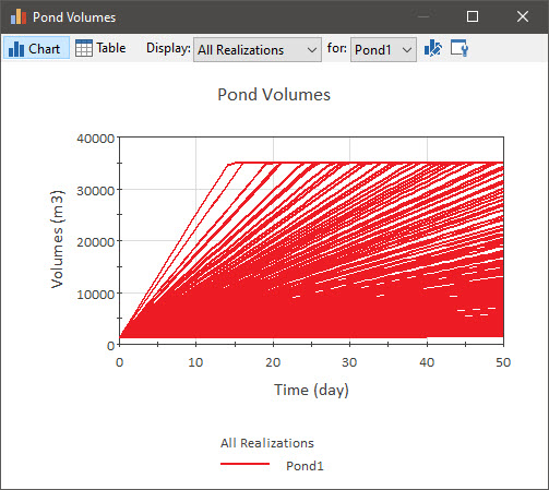
The Inflow to the pond was a Stochastic element defined as an Exponential distribution with a Mean of 500 m3/day. The Stochastic was sampled only once. Run the model again, view the Pond Volumes Time History Result element, and select “All Realizations” for the Display. You will recall that the result looks like this:
We are going to make one simple change to this model: we will assume that the Exponential distribution actually describes a frequency distribution of daily flows. Hence, we want to resample the distribution every day.
Stop now and try to build and run the model.
Once you are done with your model, save it to the “MyModels” subfolder of the “Basic GoldSim Course” folder on your desktop (call it Exercise19.gsm). If, and only if, you get stuck, open and look at the worked out Exercise (Exercise19_ Overflow_Stochastic.gsm in the “Exercises” subfolder) to help you finish the model.
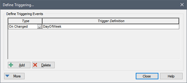
The only change to this model is to set the Stochastic to resample itself every day. The Trigger Definition should look like this:
The results (for the Pond Volumes Time History Result element, viewing “All Realizations”) looks like this:
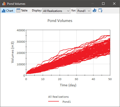
Clearly, this is a drastically different result than for when the Stochastic element was sampled only once each realization! How can we explain this? When the Stochastic was not resampled, a single value was selected and then held constant for the entire realization. Hence, if a large value was sampled for the Inflow, the Inflow was high for the entire realization (and this would result in the pond reaching its upper bound quickly). Similarly, if a small value was sampled for the Inflow, the Inflow was low for the entire realization (and this would result in the pond filling up very slowly). This resulted in a wide range of observed behaviors.
However, when the Stochastic was resampled every day, if a large value was originally sampled, the next day a new value would be sampled (and this could be low). The most likely values to be sampled would be toward the middle of the distribution. This results in behaviors that are much more closely constrained (i.e., there is much less variation between realizations).
This should make it very clear that misinterpreting what a probability distribution is intended to represent when using it in a simulation can lead to drastically different results. Hence, if you are provided with a probability distribution as input, you must very clearly understand if it represents uncertainty due to lack of knowledge (and hence should be sampled and left constant) or random temporal variation (and hence represents a stochastic process and should be resampled).
Before leaving this Exercise, let’s make one more change and rerun the model. In particular, return to Edit Mode, create another Time History Result element (name it “Inflow History”), and add the Inflow as the result to display. Then re-run the model and view that Time History Result. When you do so, set the Display to “Realization” so we can view one realization at a time. It will look similar to this:
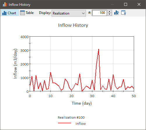
As we noted in previous Lessons, your results will look different (due to different random numbers), but the pattern will be similar. The point to note here is that every day a new value is sampled, and it is possible for the value to be very low one day and very high the next day. Knowing that in this simple example that this represents a flow rate (e.g., from a stream), you might immediately ask: “is this reasonable?” That is, does it physically make sense that the flow rate could jump around from day to day in a completely unconstrained manner? In some circumstances, perhaps it might, but in others it may not. As we will see in the next Lesson, GoldSim provides a way to represent this.
For now, save this model, as we will revisit it in the next Exercise.