Courses: Introduction to GoldSim:
Unit 13 - Probabilistic Simulation: Part II
Lesson 11 - Running a Deterministic Simulation with Uncertain Inputs
We have now covered almost everything we need to in order for you to start to take advantage of GoldSim’s probabilistic simulation features. Before we move on to other GoldSim topics, however, there is one final issue that needs to be discussed.
When you are building probabilistic models, the results can become quite complicated. After you have built your model and are trying to make probabilistic predictions, this is not a problem (and as illustrated in the last two Lessons, GoldSim provides a number of tools to help examine probabilistic results).
However, while you are constructing and testing the logic of your model, viewing probabilistic results can make it difficult to test that your model logic is correct. In general, the only way to properly test your model is to examine one realization at a time. But once you have built a probabilistic model (that includes, for example, multiple Stochastic elements and perhaps other elements that behave randomly such as time-shifted Time Series), what is the best way to do this?
One way is to simply run a single realization. You can do this by setting the # Realizations to 1 in the Monte Carlo tab of the Simulation Settings dialog:
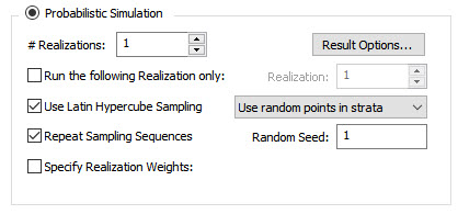
In fact, this is the default setting when you create a new GoldSim model.
Alternatively, you could choose to run a specific realization (other than the first) by checking Run the following Realization only and specifying a specific Realization. In this case, the random number sequence that is used is based on the Realization specified (and, if Latin Hypercube Sampling is used, the # Realizations). Hence, if you first run a 100 realization simulation, and then run a second simulation with Run the following Realization only checked (and, for example, Realization set to 14), the result of the second single realization simulation will be identical to the 14th realization of the first simulation. This can be useful in cases where you first run a large number of realizations (but only save a limited number of time histories) and then want to examine the details (i.e., the time history) for a particular realization for which you did not save time histories, but which exhibited some interesting behavior.
Note: In both of these cases, you would want to ensure that Repeat Sampling Sequences is on so that the realization being run is always the same during your testing.
Although running a single realization in this manner when testing your model can be valuable, it has the disadvantage that the values you are using to test the model are random. That is, when you run the single realization, GoldSim is randomly sampling the uncertain variables. This can, in some cases, make it more difficult to properly test the logic in your model.
To address this, GoldSim provides you with the ability to precisely control the values that will be used for your uncertain variables when you want to run a single realization for testing purposes. This is done by telling GoldSim to run a deterministic simulation.
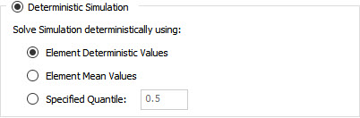
You do so by selecting the Deterministic Simulation radio button (rather than the default, Probabilistic Simulation) in the Monte Carlo tab of the Simulation Settings dialog:
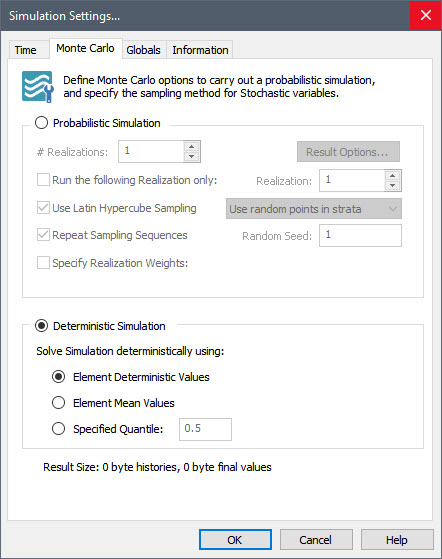
In a deterministic simulation, a single realization will be carried out using a non-random value for each Stochastic element. When you do so, it is necessary to specify what deterministic (i.e., non-random) values are to be used for each Stochastic element. As can be seen, there are three options for running a deterministic simulation:
Element Deterministic Values: In this case, the Deterministic Value explicitly specified in each individual Stochastic element property dialog is used for each Stochastic element (we will discuss this below).
Element Mean Values: In this case, the mean value of each Stochastic is used (overriding any Deterministic Value specified for each Stochastic).
Specified Quantile: In this case, the specified quantile (a number between 0 and 1) for each Stochastic is used (overriding any Deterministic Value specified for each Stochastic).
If the first option is selected (Element Deterministic Values), for each Stochastic, you must then define the Deterministic Value to be used for that specific Stochastic when a deterministic simulation is carried out. This is specified at the bottom of the dialog for each Stochastic:
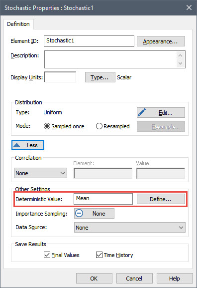
Note: To access this portion of the dialog, you may need to press the More button on the Stochastic dialog.
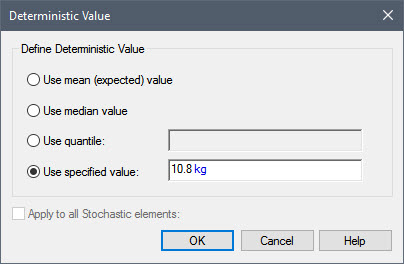
The default is for the Mean (expected) value of the Stochastic to be used as the Deterministic Value. By pressing the Define… button, however, you can specify other values:

The other options are to use the median value, use a specified quantile (e.g., 0.95), or to use a specified value (e.g., 3.7 m).
If you select one of the first three options in the dialog, you can choose to apply the selection to all Stochastics in the model (by checking the Apply to all Stochastic elements box).
If you select the fourth option (a specified value), you must specify the units when you enter the value.
In order to understand how this would work, let’s create a new model in GoldSim. Then do the following:
- Add a Stochastic element with Display Units of kg. Define it as a Normal distribution with a Mean of 10.5 kg and a Standard Deviation of 2 kg.
- Exponential distribution with a Mean of 4.5 m.
- In the Monte Carlo tab of the Simulation Settings dialog, choose to do a Deterministic Simulation, and select Element Mean Values:
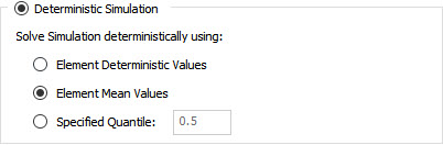
Now run the model. If you place your cursor over the first Stochastic, you will see its value is 10.5 kg. If you place your cursor over the second Stochastic, you will see that its value is 4.5 m.
Now return to Edit Mode and do the following:
- In the Monte Carlo tab of the Simulation Settings dialog, choose to do a Deterministic Simulation, but select Element Deterministic Values:
This forces GoldSim to use the specific value defined for each Stochastic. - In the first Stochastic (the Normal), change the Deterministic Value to 10.8 kg:
- In the second Stochastic (the Exponential), change the Deterministic Value to use the median:
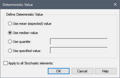
Now run the model again. If you place your cursor over the first Stochastic, you will see its value is 10.8 kg. If you place your cursor over the second Stochastic, you will see that its value is 3.12 m (which is the median value for an exponential distribution with a mean of 4.5 m).
These examples should make it clear that it is straightforward to run a single realization in which you have control over the values for the Stochastics. This will make it much easier to test complex models.
Several other points, however, should be noted regarding carrying out a Deterministic Simulation in this way:
- If you are resampling a Stochastic during a Deterministic Simulation, its value will not change (i.e., it will not behave stochastically), unless the distribution itself is changed as a function of time. Hence, if stochastic behavior is critical to see while testing your model, you would need to run a Probabilistic Simulation with a single realization.
- Stochastic elements are not the only elements that behave probabilistically. Other elements in GoldSim also do so (e.g., randomly time-shifted Time Series elements, which we discussed in Lesson 6, and Event elements, which we will discuss in Unit 14). In a Deterministic Simulation, these elements also behave deterministically (i.e., their behavior is no longer random). For example, for the case of a time-shifted Time Series, GoldSim samples the time series from the middle of the historic data (the sampling is based on the median value of the series).
- You may recall that when running a probabilistic simulation with multiple realizations, you can view various time history and final value statistics, including the mean. It is important to understand that the mean result in a probabilistic simulation is not the same as the result of deterministic simulation in which mean values have been used for the uncertain variables. These are two completely different results and should never be confused! That is, the mean of function (e.g., a simulation) IS NOT the same as the function of the means. The only way to compute the mean (e.g., expected) value of a complex function (e.g., a simulation) is to run the model for multiple realizations and compute the mean based on those realizations.