Courses: Introduction to GoldSim:
Unit 16 - Documenting Your Model
Lesson 7 - Customizing the Appearance of Elements
Another option provided by GoldSim for helping to document your model is the ability to customize the symbol that is used in the graphics pane to represent an element. Under what circumstances would you want to do that?
The symbols for the GoldSim elements were specifically designed to act as visual cues so that (if the model is well organized) someone can begin to understand the model just by looking at the graphics pane. The Sum and Extrema elements are particularly good examples of this. You will also note that elements of a particular type or category share some features or color. For example, Input elements are green; Stock elements are orange; event elements tend to have “sharp” edges rather than a uniform shape. All of these conventions are designed to make your models easier to understand. As a result, as a general rule, you would rarely want to change the appearance of the (non-Container) elements symbols at lower levels (i.e., deep in the containment hierarchy) of your models, as the symbols serve an important purpose.
However, the higher level portions of your models will often consist a number of Containers. The Container symbol itself does provide a visual cue (since it is a box) that it represents a sub-system. However, all Containers also have a small triangle in their upper left-hand corner that also identifies them as a Container. As a result, Containers are always be easy to recognize regardless of their symbol.
Moreover, because Containers often represent sub-systems of the model, customizing their symbol to better represent what is actually being represented inside the Container can make the model easier to understand. To illustrate that, consider the following model:
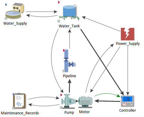
All of the symbols for these elements have been customized. All but one (Power_Supply) are Containers.
So we see that customizing the element symbols can be a powerful way to make your model easier to understand (and in many cases, more interesting and attractive). So how do we do that in GoldSim? Let’s experiment with that now.
The first thing you must understand is that if you wish to replace a symbol, you can replace it with a custom symbol, but the image file must be an enhanced Windows metafile plus (.emf) file. GoldSim utilizes enhanced metafiles (emf) for element symbols because they are vector graphics (and therefore scale without losing image quality). Most advanced graphics programs can create enhanced metafiles (or convert other formats to an enhanced metafile). Note, however, that when converting other formats to emf files, unless the original image was created using a vector format (and is converted properly), it will lose image quality when scaling in GoldSim.
Let’s walk through the process of changing a symbol now. Start with a new file, and insert a Container element. We are going to replace the default symbol with a custom symbol (that you will find in the “Examples” subfolder of the “Basic GoldSim Course” folder you should have downloaded and unzipped to your Desktop).
To do so, do the following:
- Right-click on the element, and select Appearance… to display this dialog:
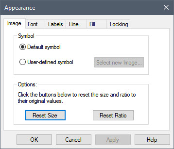
- Select User-defined symbol, and you will be prompted for a file. Navigate to the “Examples” subfolder of the “Basic GoldSim Course” folder you should have downloaded and unzipped to your Desktop and select the file named WaterTank.emf.
- If the new image is a different size than the old image (which will typically be the case, and is the case here), you will be asked whether you want to adjust the size of the new image to match the size of the existing element or to adjust the size of the element to match the size of the new image. In this case, answer Yes.
- Close the Appearance dialog.
The Container now looks like this:

Once the image for the element is defined using a user-defined symbol, you can change the symbol by pressing Select new Image…, or you can switch back to the default image provided by GoldSim by selecting the Default symbol radio button (do that now).
You can also change or reset the images for multiple elements in a model (e.g., all elements of one type) by selecting Graphics|Change Symbols… from the main menu. If you are interested, insert another Container (so there are two), and explore that option now.
Note: You can also change the symbol for a Hyperlink object (discussed in the previous Lesson). That is, by right-clicking on a Hyperlink, you can access an Appearance dialog.