Lesson 2 - Representing a Spatially Continuous Transport Process in GoldSim

Before discussing the process of diffusion in detail, let’s first revisit a very simple advective system we touched on very briefly in Unit 3, as it provides a nice introduction to how we will represent a spatially continuous transport process.

Imagine we have a horizontal tube of cross-sectional area A and length L in which water enters at one end and exits at the other end:

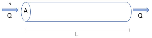
In this case, if we introduced mass into the at the upstream end at a constant concentration S (uniformly across the entire cross-sectional area), the concentration would subsequently vary continuously along the tube from 0 to L.  Let’s assume that we can treat the system as fully one-dimensional (i.e., the flow rate and the concentration is constant across a cross-sectional plane normal to the flow). Let’s also assume that the mass moves though the tube as “plug flow”.  That is, there is no mixing, dispersion or diffusion as it flows through the tube and a “plug” of equal concentration moves through the tube (at a velocity of v). This is a purely advective system. In this case, it can be shown that we could write the governing equation describing that concentration as follows:

v is the velocity of the flowing water (equal in this simple example to Q/A, where Q is the flow rate and A is the cross-sectional area), and x is the distance along the tube  (from 0 to L). (To fully describe this system, we would also need to specify boundary conditions at the upstream and downstream ends of the tube, but for the purposes of the present discussion, we don’t need to worry about this.) Note that this is a partial differential equation, in that C is a function of both time and distance along the tube.

If we assume that this equation is appropriate (i.e., mass moves through the system as “plug flow”), then if we were to monitor the concentration at the end of the tube (at x = L) we would find that the concentration would jump (in a vertical line) from zero to the source concentration (S) at a time equal to L/v:

How can we represent a system like this and numerically solve it in GoldSim? One approach we might take (and the one we will discuss in great detail later in this Unit when we consider diffusive transport and the next Unit, when we consider advective-dispersive transport) would be to spatially discretize the system into a series of finite volumes, effectively chopping the tube up into sections. We can actually do this using the mixing Cells we have been discussing in previous Units. To see this, let’s open a model that shows how this can be done.  Go to the “Examples” subfolder of the “Contaminant Transport Course” folder you should have downloaded and unzipped to your Desktop, and open a model file named ExampleCT17_Plug_Flow.gsm.

This particular model has a single species (X).  The values for the variables discussed above are as follows (you can find these in the Inputs Container):

• L = 10 m
• A = 1 m2
• Q = 1 m3/min
• S = 10 mg/l

As pointed out above, the concentration should jump (in a vertical line) from zero to 10 mg/l at a time equal to L/v. Since v = Q/A, L/v is equal to 10 min.

If we look at the Tube Container, we can see how we have simulated this:

We have represented the tube as a series of 10 Cells. Each Cell, of course, is well-mixed (and as we shall see, that will have important consequences). If we look at any given Cell (e.g., Cell2), we see that the volume of water represents 1/10th of the volume of the entire tube:

Cell2 has a single outflow:

It also has a single inflow (from Cell1):

There are two additional Cells here. The Source Cell simply provides a constant Defined Concentration (S) flowing into the tube. The Sink Cell provides the sink into which the tube flows.

So we have represented this system using the Cell pathways that we have been discussing in previous Units. In this case, however, we are trying to use them to represent a spatially continuous transport process. We are doing this by spatially discretizing the tube (in this case, into 10 “slices”).  Will this work? 

Run the model and double-click on the Concentration Result element:

This plots the concentration leaving the tube (actually, the concentration in Cell10), as well as the analytical result.  As we can see, the simulated result is not very close to the analytical result at all.  The simulated result is “smeared” or spread out over time (rather than being a vertical step).

So what is happening here?  What this example illustrates is the problem of numerical diffusion. This is not real diffusion; it is an artefact of the numerical solution method. Conceptually, this results from the fact that each of the 10 Cells is well-mixed.  So when mass enters a Cell, it is instantaneously mixed across the full length of the Cell (in this case, each Cell represents 10% of the tube). This results in a spreading of the mass.  As you might imagine, we can decrease the amount of numerical diffusion by increasing the level of spatial discretization (e.g., using 100 Cells instead of 10 Cells).  Even with 100 Cells in this example, however, we would still have noticeable spreading. 

Representing sharp breakthrough curves like this is computationally difficult to do numerically. Fortunately, it is almost never necessary to do so in actual mass transport models.  This is because in the real world, there is indeed significant spreading due to physical dispersion (discussed in Unit 3, Lesson 4).  As we will discuss in the next Unit, there are ways we can adjust the representation here to explicitly model these dispersive processes.  We then simply need to make sure that the artificial numerical diffusion is less than the actual dispersion we are trying to represent (by adjusting the level of discretization). 

In this Unit we are not discussing an advective process like in this tube example, but a diffusive process. We have started with this advective tube example, however, because, as we will see, like in this tube example, we will simulate diffusion by using Cells to spatially discretize the system through which diffusion is occurring.  And like the tube example discussed above, this discretization will result in some error (with the amount of error decreasing as the amount of discretization increases). As a result, we will need to select our discretization in such a way that we can represent the actual diffusive process with sufficient accuracy.