Lesson 2 – Understanding the Advection-Dispersion Equation

In Unit 3, we introduced a simple example of a system we can describe using the advection-dispersion equation. Let’s revisit that (with a small modification) now.

Imagine we have a horizontal tube of cross-sectional area A and length L which is filled with a porous medium (e.g., sand) and is completely saturated with water.  We will further assume water enters at one end and exits at the other end:

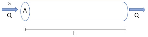
In this case, if we introduced mass into the tube at the upstream end at a constant concentration S (uniformly across the entire cross-sectional area), the concentration would subsequently vary continuously along the tube from 0 to L.  Let’s assume that we can treat the system as fully one-dimensional (i.e., the flow rate and the concentration is constant across a cross-sectional plane normal to the flow). Let’s also assume that the mass moves though the tube as “plug flow”.  That is, there is no mixing, dispersion or diffusion as it flows through the tube and a “plug” of equal concentration moves through the tube (at a velocity of v). This is a purely advective system. In this case, it can be shown that we could write the governing equation describing that concentration as follows:

where v is the seepage velocity of the flowing water (equal in this simple example to Q/ (n A), where Q is the flow rate, A is the cross-sectional area, and n is the porosity of the sand), and x is the distance along the tube (from 0 to L). (To fully describe this system, we would also need to specify boundary conditions at the upstream and downstream ends of the tube, but for the purposes of the present discussion, we don’t need to worry about this.) Note that this is a partial differential equation, in that C is a function of both time and distance along the tube. We can refer to this as the advection equation.

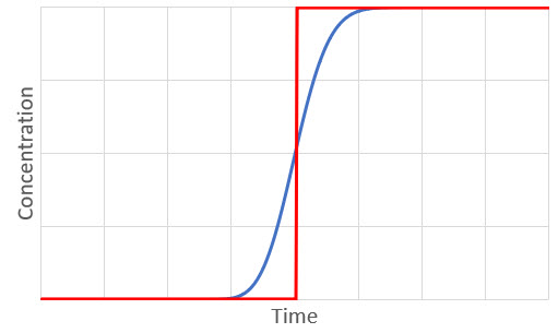
If we assume that this equation is appropriate (i.e., mass moves through the system as “plug flow”), then if we were to monitor the concentration at the end of the tube (at x = L) we would find that the solution to this equation would indicate that concentration would jump (in a vertical line) from zero to the source concentration (S) at a time equal to L/v. However, if we were to actually run a real experiment, we would find that the observed concentration leaving the tube would not behave this way at all. Instead, we would see that this breakthrough would be spread out or dispersed to some extent (as shown schematically by the blue curve below). That is, realistically, we can’t explain the behavior using advection alone and need to also represent whatever process is causing this dispersion.

Molecular diffusion can cause some mixing like this.  But generally the effect of diffusion would be very small (the spreading would be minor). For flow through porous media, the fluid is generally moving slowly and is not turbulent (so that is not what is causing this dispersion). But the groundwater must take detours around the various solid particles, and these detours result in mixing, referred to as mechanical dispersion (or hydrodynamic dispersion). This is what would cause the spreading we would observe in the tube. Particularly in a large-scale environmental system (e.g., a groundwater aquifer) this kind of dispersion can also take place at a larger scale than that of the individual particles, as water may flow around large-scale regions of less permeable material (referred to as macrodispersion).  Like molecular diffusion, mechanical dispersion has the effect of transporting mass in the direction of decreasing concentration.

Adding these processes to the advection equation yields the (one-dimensional) advection-dispersion equation (for a saturated porous medium):

where D_m is the molecular diffusion coefficient and D is the mechanical dispersion coefficient (both have dimensions of L2/T). (The variable t is the tortuosity and n is the porosity of the porous medium). By definition, if the system is advectively-dominated (the systems we will consider in this Unit), the molecular diffusion coefficient can generally be ignored (as it is much smaller than D).

D is often approximated as:

where α is the (longitudinal) dispersivity (dimensions of L). The dispersivity is often treated as scale-dependent.  That is, it is treated as a function of the length scale of the problem (e.g., 10% of the total length of the tube).

As we shall see in this Unit, GoldSim provides two alternative ways to solve the one-dimensional advection-dispersion equation. One (used by an element called a Pipe pathway) can be thought of as an analytical approach using Laplace transforms. Laplace transforms solve differential equations by converting them into algebraic equations. We won’t go into any further detail in this Course on how Laplace transforms do this (you can read about this in any differential equations textbook if you are curious).  For the purposes of this Course, you can simply view it as an approach that solves the equation without requiring use of spatial discretization.

The other approach for solving this differential equation (used by an element called an Aquifer pathway) involves using a finite difference approximation in the same manner that we did when solving ordinary differential equations for well-mixed compartments.  However, now instead of approximating only the time derivative using finite differences, we must also approximate the spatial derivatives. To do so, we must not only discretize time, but we must also discretize space. The finite difference approximation to the equation looks like this:

In this equation, the tube has been discretized spatially into a fixed number of finite volumes (of length Δx). The equation involves the concentration in three adjacent volumes: j, j-1 (which is immediately upgradient of j) and j+1 (which is immediately downgradient of j). The superscript k refers to the timestep (k is the current timestep k-1 is the previous timestep, and Δt is the timestep length). There is an equation for every volume so, for example, if the tube was divided into 20 finite volumes, there would be 20 equations with 20 unknowns for each contaminant being modeled. 

These equations could be rewritten in terms of the mass in each volume (rather than the concentration). After doing so, this system of equations would look very similar to the equations for advection through a series of well-mixed tanks (e.g., like what we discussed in Unit 6).  The equations for the Aquifer, however, are more tightly coupled than those for the tanks.  This is because for the Aquifer, each equation would reference its own mass, the mass in the finite volume upstream, and the mass in the finite volume downstream. For the tanks, however,  each equation would reference its own mass and the mass in the finite volume upstream, but would not reference the mass in the finite volume downstream.  However, the equations for the Aquifer are still linear, and can be solved in the same way. As we will see, the degree to which space is discretized (i.e., how many finite volumes are used) is consequential and must be selected with care.

Each of these two approaches to solving the advection-dispersion equation has its advantages and disadvantages.  We will discuss both approaches in detail in the remainder of this Unit, starting with the latter approach (that used by the Aquifer element).