Lesson 3 – Introduction to the Aquifer Pathway

In this Lesson, we are going to introduce the Aquifer element. To do so, we are going to walk through the simple system described in the previous Lesson - a horizontal tube filled with saturated sand:

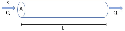
Recall that the tube has cross-sectional area A and length L, and is filled with a porous medium (sand with porosity n and bulk density rho) and is completely saturated with water.  Water enters at one end and exits at the other end (at a flow rate of Q and velocity v). The water introduced at the upstream end of the tube (uniformly across the entire cross-sectional area) contains two species (X and Y) at a constant concentration S. One of the species (Y) partitions onto the sand, while the other does not. The degree of dispersion is quantified in terms of the (longitudinal) dispersivity (alpha).

Go to the “Examples” subfolder of the “Contaminant Transport Course” folder you should have downloaded and unzipped to your Desktop, and open a model file named ExampleCT25_Aquifer.gsm.  The model looks like this:

The values for the variables discussed above are as follows (you can find these in the Inputs Container):

• L = 10 m
• A = 1 m2
• Q = 1 m3/min
• S = 10 mg/l
• n = 0.3
• rho = 1600 kg/m3
• alpha = 1m
• K_d for Y = 1.88 E-4 m3/kg (the Kd for X is zero).

Let’s first open the Aquifer element (named Tube):

The first two input fields in the Aquifer pathway dialog describe the overall geometry of the pathway: 

• Length:  This is the length of the pathway.
• Area:  This is the total cross-sectional area of the pathway. In this particular Example model, the appropriate Area to specify is obvious, but in other kinds of models, it may not be. Hence, we will discuss this further in the next Lesson.

In addition to the inputs describing Aquifer geometry, Aquifers require four additional inputs that control their behavior:

• Dispersivity:  This is the longitudinal dispersivity of the pathway. It has dimensions of length. It is typically defined in terms of a fraction of the total pathway length (i.e., it scales with the length of the pathway to represent macrodispersion). A good first approximation for one-dimensional transport through a relatively homogeneous porous medium might be that the dispersivity is 10% to 30% of the total length of the pathway.
• Number of Cells:  As noted in the previous Lesson, the Aquifer element solves the advection-dispersion equation by using a finite difference approximation that involves discretizing the pathway into a series of finite volumes. This represents the number of finite volumes that are used. We will discuss this input in detail in Lesson 5.
• Infill Medium:  This is the (optional) porous medium that fills the (entire) pathway.  It must be an existing Solid medium in the model.  You can, however, specify that there is no porous medium filling the pathway (e.g., if you were simulating a tube with no sand, or perhaps a stream) by leaving this field blank. The porous medium affects the behavior of the Aquifer in two ways: 1) for a given flow rate, it increases the flow velocity (by reducing the effective flow area); and 2) it can act to retard any species that partition onto it.  We will discuss both of these effects below when we examine the results.
• Fluid Saturation:  This is the degree of saturation of the Aquifer.  It is dimensionless, and must be greater than 0 and less than or equal to 1.  If you were simulating flow through a saturated porous medium (as we are here), you would specify the fluid saturation as 1 (the default).  If, however, you were simulating flow through an unsaturated porous medium (e.g., surface soils or a vadose zone), this would be specified as less than 1. We will discuss this further in the next Lesson.

The Input Rate input is a selection from a drop-list that provides three options for adding mass to the pathway:

• Initial Inventory: An initial amount of mass is applied at the beginning (the first finite volume) of the pathway.
• Input Rate: The specified rate (which can change with time) is applied at the beginning (the first finite volume) of the pathway. This is the option selected in this Example.
• Cumulative Input: This option provides a mechanism for simultaneously specifying an initial condition and a rate of mass addition (that may change with time).

These options are analogous to those provided for a Cell as discussed in Unit 6, Lesson 8 (the Aquifer pathway, however, does not include an option for a Defined Concentration). In this example, the Input Rate is defined as the constant flow rate multiplied by the constant concentration.

We will discuss the Source Zone Length input and the Enable dispersive and diffusive outfluxes… checkbox in Lesson 7 and the Suspended Solids button in Lesson 11.  None of them apply to this simple Example.

Now select the Outflows tab:

You will note that this looks identical to the Outflows tab for a Cell. In fact, the Inflows and Outflows tabs for an Aquifer are identical to those for a Cell. However, you can create only advective mass flux links from an Aquifer. The specialized mass flux links we discussed in Unit 7 (Lessons 10 and 11) and the diffusive mass flux links we discussed in Unit 8 cannot originate from an Aquifer (although they can be linked to an Aquifer). In this Example, you will see that we have created an advective mass flux link to a Sink Cell.  The Flow Rate is the flow rate in the Aquifer. All Aquifers must have at least one advective mass flux link to another pathway with a positive Flow Rate defined: it is the only way to define the flow rate through the Aquifer. Otherwise, GoldSim will generate a fatal error message.

There is one other thing worth noting here about the advective mass flux link from the Aquifer to the Cell: it is necessarily a Normal link.  You should recall our discussion regarding the different types of mass flux links from Unit 6, Lesson 11. We noted that Cells by default use Coupled links.  You cannot, however, create a Coupled link to or from an Aquifer pathway (because the mathematical representation of the Aquifer is its own system of coupled equations).  By default, they are Normal links (although as we will discuss in Lesson 12, they can also be specified as Previous-value links).

Close the dialog and left-click on the output port for the Aquifer:

There are three outputs here. Mass_in_Pathway is the total mass in the Aquifer (which generally is not a very interesting result, as this mass is spread out over the entire pathway).  Concentration is the concentration leaving the pathway. The Outflows folder contains mass transfer rates for all of the advective mass flux links leaving the pathway (in this case, we have only one).

Run the model and double-click on the “Concentration Leaving Tube” Result element:

What we see is that mass moves through the pathway (and is dispersed). Both species eventually breakthrough completely such that the concentration leaving the tube is the same as the concentration entering.  This breakthrough takes longer for Y since it partitions onto the sand as it moves through the tube.

The expected travel time through the tube (which can also be thought of as the travel time in the absence of dispersion), can be computed as follows:

Expected Travel Time = n A L/Q

Using the values for this Example, this can be calculated to be equal to 3 minutes.  As can be seen, for species X (which does not partition onto the sand), the concentration actually reaches 50% of its final value a little before 3 minutes.  This is because the nature of the equation (and boundary conditions) is such that unless the dispersivity is very small, the breakthrough is asymmetric. Nevertheless, the expected travel time calculation still provides a rough approximation of the “center” of the breakthrough. 

Note that species Y is delayed by a factor of two (if you look at any given concentration for X, it takes twice as long to reach the same concentration for Y). This is a direct result of partitioning onto the sand.  A retardation factor resulting from this partitioning can be computed as follows:

Retardation factor = 1 + (rho K_d/n)

Using the values for this Example, this can be calculated to be equal to 2.

Now that we have provided a basic introduction to the Aquifer element, in the next Lesson we will discuss in more detail how the inputs are specified.